cell_typing

Cell typing by data integration and by classification¶

Here, we walk you through three ways to predict the cell types in your query scRNAseq data set by leveraging another, well-annotated reference dataset. The first way is to directly combine the datasets and cluster them together. The second way is called 'Batch Balanced KNN', which works by finding kNN across batches. The third way is to classify the query data with classifier that was trained with the reference data.

Data¶

We will use mouse cells from gastrula-stage embryos from two studies.

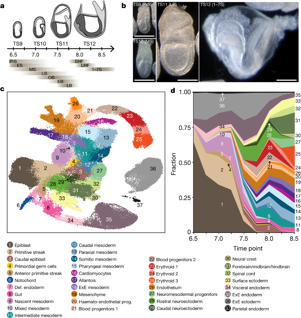
The reference data comes from Pijuan-Sala et al 2019 which describes a single cell census of gastrulation in mouse (E6.5 to E8.5). You can download the .h5ad file here.

A single-cell resolution atlas of mouse gastrulation and early organogenesis. Fig 1 from Pijuan-Sala et al 2019

The query data comes from another gastrula census Grosswendt et al 2020. You can download the .h5ad file here.

For the sake of computational efficiency, we have taken only a small subset of the cells from each of these studies. The cell type label is stored in .obs['celltype']

Environment setup¶

Local (conda): Create the environment from the provided cell_typing_integration_environment.yml:

conda env create -f cell_typing_integration_environment.yml
conda activate cscb

Pip only: Use cell_typing_integration_requirements.txt:

pip install -r cell_typing_integration_requirements.txt

Google Colab: Run the cell below — it will detect Colab and install the required packages automatically. You will also need to upload the data files to data/ in your Colab working directory.

In [28]:

import sys
if 'google.colab' in sys.modules:
    print("Colab detected — installing required packages...")
    !pip install -q scanpy==1.10.3 anndata==0.11.1 bbknn==1.6.0 pySingleCellNet==0.1.3 leidenalg==0.10.2 igraph==0.11.8
else:
    print("Local environment detected — skipping install.")

import sys if 'google.colab' in sys.modules: print("Colab detected — installing required packages...") !pip install -q scanpy==1.10.3 anndata==0.11.1 bbknn==1.6.0 pySingleCellNet==0.1.3 leidenalg==0.10.2 igraph==0.11.8 else: print("Local environment detected — skipping install.")

Local environment detected — skipping install.

In [29]:

import warnings
warnings.filterwarnings("ignore", category=FutureWarning)
import os, sys
import numpy as np
import pandas as pd
import matplotlib.pyplot as plt
import scanpy as sc
import pySingleCellNet as cn
import scanpy.external as sce
print(sys.executable)

import warnings warnings.filterwarnings("ignore", category=FutureWarning) import os, sys import numpy as np import pandas as pd import matplotlib.pyplot as plt import scanpy as sc import pySingleCellNet as cn import scanpy.external as sce print(sys.executable)

/opt/homebrew/Caskroom/miniforge/base/envs/cscb/bin/python

In [30]:

import bbknn
print(f"bbknn version: {bbknn.__version__}")

import bbknn print(f"bbknn version: {bbknn.__version__}")

bbknn version: 1.6.0

In [31]:

data_path = "../../data/"
adPijuan = sc.read_h5ad(data_path + "ad_Pijuan_demo.h5ad")
adPijuan

data_path = "../../data/" adPijuan = sc.read_h5ad(data_path + "ad_Pijuan_demo.h5ad") adPijuan

Out[31]:

AnnData object with n_obs × n_vars = 2071 × 21133
    obs: 'cell', 'stage', 'celltype'
    var: 'ENSEMBL'

In [32]:

adPijuan.obs['celltype'].value_counts()

adPijuan.obs['celltype'].value_counts()

Out[32]:

celltype
Meso.Cardio     300
PGC             297
Endo.Gut        296
Epiblast        296
Anterior.PS     294
Ecto.Neural     294
Meso.Nascent    294
Name: count, dtype: int64

Standard pre-processing pipeline

In [33]:

adTrain = adPijuan
adTrain.layers['counts'] = adTrain.X.copy()
sc.pp.normalize_total(adTrain)
sc.pp.log1p(adTrain)
# Or choose your preferred HVG 
sc.pp.highly_variable_genes(adTrain, n_top_genes=2000, flavor='seurat_v3', layer='counts')

adTrain = adPijuan adTrain.layers['counts'] = adTrain.X.copy() sc.pp.normalize_total(adTrain) sc.pp.log1p(adTrain) # Or choose your preferred HVG sc.pp.highly_variable_genes(adTrain, n_top_genes=2000, flavor='seurat_v3', layer='counts')

In [34]:

sc.tl.pca(adTrain, mask_var='highly_variable')
sc.pl.pca_variance_ratio(adTrain, n_pcs=50)

sc.tl.pca(adTrain, mask_var='highly_variable') sc.pl.pca_variance_ratio(adTrain, n_pcs=50)

kNN and then UMAP for visualization

In [35]:

def_npcs = 20
def_nneigh = 10
sc.pp.neighbors(adTrain, n_neighbors = def_nneigh,  n_pcs = def_npcs)

def_npcs = 20 def_nneigh = 10 sc.pp.neighbors(adTrain, n_neighbors = def_nneigh, n_pcs = def_npcs)

Color cells by ground truth label and by developmental stage

In [36]:

sc.tl.umap(adTrain)
sc.pl.umap(adTrain, color=['celltype', 'stage'], size=30, alpha=.95,frameon=False)

sc.tl.umap(adTrain) sc.pl.umap(adTrain, color=['celltype', 'stage'], size=30, alpha=.95,frameon=False)

Naive concatenation of anndata objects, then clustering¶

Now we will load the other scRNAseq data set from another study that also looked at mouse gastrulation.

In [37]:

adGross = sc.read_h5ad(data_path + "ad_Grosswendt_demo.h5ad")
adGross

adGross = sc.read_h5ad(data_path + "ad_Grosswendt_demo.h5ad") adGross

Out[37]:

AnnData object with n_obs × n_vars = 700 × 21133
    obs: 'embryo', 'stage', 'celltype'
    var: 'name'

In [38]:

adPijuan = sc.read_h5ad(data_path + "ad_Pijuan_demo.h5ad")
adPijuan.obs['study'] = 'Pijuan'
adGross.obs['study'] = 'Grosswendt'

adPijuan = sc.read_h5ad(data_path + "ad_Pijuan_demo.h5ad") adPijuan.obs['study'] = 'Pijuan' adGross.obs['study'] = 'Grosswendt'

In [39]:

import anndata as ad
del(adPijuan.raw)
adComb = ad.concat([adPijuan, adGross])

import anndata as ad del(adPijuan.raw) adComb = ad.concat([adPijuan, adGross])

In [40]:

adComb.obs['study'].value_counts()

adComb.obs['study'].value_counts()

Out[40]:

study
Pijuan        2071
Grosswendt     700
Name: count, dtype: int64

In [41]:

adComb.layers['counts'] = adComb.X.copy()
sc.pp.normalize_total(adComb)
sc.pp.log1p(adComb)
sc.pp.highly_variable_genes(adComb, n_top_genes=2000, flavor='seurat_v3', layer='counts')
sc.tl.pca(adComb, mask_var='highly_variable')
sc.pl.pca_variance_ratio(adComb, n_pcs=50)

adComb.layers['counts'] = adComb.X.copy() sc.pp.normalize_total(adComb) sc.pp.log1p(adComb) sc.pp.highly_variable_genes(adComb, n_top_genes=2000, flavor='seurat_v3', layer='counts') sc.tl.pca(adComb, mask_var='highly_variable') sc.pl.pca_variance_ratio(adComb, n_pcs=50)

In [42]:

sc.pl.pca(adComb, color=['study', 'celltype'], size=30, alpha=.95,frameon=False)

sc.pl.pca(adComb, color=['study', 'celltype'], size=30, alpha=.95,frameon=False)

In [43]:

def_npcs = 20
def_nneigh = 10 # my preference -- lower values tend to facilitate detection of rarer populations
sc.pp.neighbors(adComb, n_neighbors = def_nneigh,  n_pcs = def_npcs)
sc.tl.umap(adComb)
sc.pl.umap(adComb, color=['study', 'celltype'], size=30, alpha=.95,frameon=False)

def_npcs = 20 def_nneigh = 10 # my preference -- lower values tend to facilitate detection of rarer populations sc.pp.neighbors(adComb, n_neighbors = def_nneigh, n_pcs = def_npcs) sc.tl.umap(adComb) sc.pl.umap(adComb, color=['study', 'celltype'], size=30, alpha=.95,frameon=False)

The embedding above strongly suggests that cells clustering will be dominated by study over cell type. Let's test this...

In [44]:

sc.tl.leiden(adComb, 0.25, flavor="igraph", n_iterations=2, directed=False)
sc.pl.umap(adComb, color=['study', 'celltype', 'leiden'], size=30, alpha=.95,frameon=False)

sc.tl.leiden(adComb, 0.25, flavor="igraph", n_iterations=2, directed=False) sc.pl.umap(adComb, color=['study', 'celltype', 'leiden'], size=30, alpha=.95,frameon=False)

Method 2: BBKNN¶

Let's test Batch Balanced K Nearest Neighbors (BBKNN) (Polanski et al 2020), a graph-based integration method. Rather than aligning expression values across batches, BBKNN modifies the KNN graph construction step so that each cell's neighbors are balanced across batches. This corrected graph is then used for downstream steps like UMAP and clustering.

For details on how the sc.external.pp.bbknn() function works, see scanpy's documentation.

Also see the section on graph-based integration in the online best practices book.

If bbknn is not already installed in your environment, install it with:

pip install bbknn

See https://github.com/Teichlab/bbknn for more details. Note: bbknn >= 1.6.0 is required for compatibility with scikit-learn >= 1.3.

In [45]:

adComb2 = ad.concat([adPijuan, adGross])
batch_key = "study"

sc.pp.filter_genes(adComb2, min_cells=3)
adComb2.layers['counts'] = adComb2.X.copy()

adComb2 = ad.concat([adPijuan, adGross]) batch_key = "study" sc.pp.filter_genes(adComb2, min_cells=3) adComb2.layers['counts'] = adComb2.X.copy()

In [46]:

sc.pp.normalize_total(adComb2)
sc.pp.log1p(adComb2)
sc.pp.highly_variable_genes(adComb2, n_top_genes=2000, flavor="cell_ranger", batch_key=batch_key)

sc.pp.normalize_total(adComb2) sc.pp.log1p(adComb2) sc.pp.highly_variable_genes(adComb2, n_top_genes=2000, flavor="cell_ranger", batch_key=batch_key)

In [47]:

adata_hvg = adComb2[:,adComb2.var["highly_variable"]].copy()
sc.pp.pca(adata_hvg)
sce.pp.bbknn(adata_hvg, batch_key=batch_key)

adata_hvg = adComb2[:,adComb2.var["highly_variable"]].copy() sc.pp.pca(adata_hvg) sce.pp.bbknn(adata_hvg, batch_key=batch_key)

WARNING: consider updating your call to make use of `computation`

In [48]:

adata_hvg

adata_hvg

Out[48]:

AnnData object with n_obs × n_vars = 2771 × 2000
    obs: 'stage', 'celltype', 'study'
    var: 'n_cells', 'highly_variable', 'means', 'dispersions', 'dispersions_norm', 'highly_variable_nbatches', 'highly_variable_intersection'
    uns: 'log1p', 'hvg', 'pca', 'neighbors'
    obsm: 'X_pca'
    varm: 'PCs'
    layers: 'counts'
    obsp: 'distances', 'connectivities'

In [49]:

sc.tl.umap(adata_hvg)
sc.pl.umap(adata_hvg, color=['study', 'celltype'], size=30, alpha=.95,frameon=False)

sc.tl.umap(adata_hvg) sc.pl.umap(adata_hvg, color=['study', 'celltype'], size=30, alpha=.95,frameon=False)

The integration by BBKNN in this example looks pretty good! Note that in both this approach and the naive integration, the user would still need to perform some post-integration processing in order to label the query cells. This could easily be done by clustering and then assigning query cells based on the most frequent label of reference cells sharing the same cluster as query cells. Try to think of other approaches to this task.

Method 3: ML Classification¶

In the third approach, we will directly annotate query cells by classifying them using a model trained on reference data. Our PySingleCellNet (pySCN) package was designed for this task (Tan and Cahan 2019). SingleCellNet trains a random forest classifier on gene expression features derived from the reference data, and then applies it to classify query cells. It also includes tools to assess classification performance and to categorize predictions by confidence.

In [50]:

adRef2 = sc.read_h5ad(data_path + "ad_Pijuan_demo.h5ad")
adQuery = sc.read_h5ad(data_path + "ad_Grosswendt_demo.h5ad")

adRef2 = sc.read_h5ad(data_path + "ad_Pijuan_demo.h5ad") adQuery = sc.read_h5ad(data_path + "ad_Grosswendt_demo.h5ad")

In [51]:

cn.ut.limit_anndata_to_common_genes([adRef2, adQuery])

cn.ut.limit_anndata_to_common_genes([adRef2, adQuery])

In [52]:

n_cells = 100
groupby = 'celltype'
# Stratify the train/validation split by developmental stage so both sets have balanced stage representation
strata_col = 'stage'

tids, vids = cn.ut.split_adata_indices(adRef2, n_cells, groupby=groupby, cellid=None, strata_col=strata_col)

n_cells = 100 groupby = 'celltype' # Stratify the train/validation split by developmental stage so both sets have balanced stage representation strata_col = 'stage' tids, vids = cn.ut.split_adata_indices(adRef2, n_cells, groupby=groupby, cellid=None, strata_col=strata_col)

In [53]:

adTrain = adRef2[tids].copy()
adHO = adRef2[vids].copy()

adTrain = adRef2[tids].copy() adHO = adRef2[vids].copy()

In [54]:

sc.pp.highly_variable_genes(adTrain, n_top_genes=3000, flavor='seurat_v3')
sc.pp.normalize_total(adTrain)
sc.pp.log1p(adTrain)

sc.pp.highly_variable_genes(adTrain, n_top_genes=3000, flavor='seurat_v3') sc.pp.normalize_total(adTrain) sc.pp.log1p(adTrain)

In [55]:

n_rand = n_cells
n_top_genes = 30
n_top_gene_pairs = 40
n_comps = 30
n_trees = 1000
obs_pred = "SCN_class_argmax"

clf = cn.tl.train_classifier(adTrain, groupby, n_rand=n_rand, n_top_genes=n_top_genes, n_top_gene_pairs=n_top_gene_pairs, n_comps=n_comps)

n_rand = n_cells n_top_genes = 30 n_top_gene_pairs = 40 n_comps = 30 n_trees = 1000 obs_pred = "SCN_class_argmax" clf = cn.tl.train_classifier(adTrain, groupby, n_rand=n_rand, n_top_genes=n_top_genes, n_top_gene_pairs=n_top_gene_pairs, n_comps=n_comps)

Training classifier |████████████████████████████████████████| 5/5 [100%] in 2.2s (2.29/s) 

In [56]:

cn.tl.classify_anndata(adHO, clf)

cn.tl.classify_anndata(adHO, clf)

In [57]:

adHO

adHO

Out[57]:

AnnData object with n_obs × n_vars = 1386 × 21133
    obs: 'cell', 'stage', 'celltype', 'cellid', 'SCN_class_argmax'
    var: 'ENSEMBL'
    uns: 'SCN_class_argmax_colors'
    obsm: 'SCN_score'

In [58]:

type(adHO.obsm)

type(adHO.obsm)

Out[58]:

anndata._core.aligned_mapping.AxisArrays

In [59]:

adHO.obsm

adHO.obsm

Out[59]:

AxisArrays with keys: SCN_score

In [60]:

cn.pl.heatmap_scores(adHO, groupby = 'SCN_class_argmax')

cn.pl.heatmap_scores(adHO, groupby = 'SCN_class_argmax')

In [61]:

cn.pl.heatmap_scores(adHO, groupby = 'celltype')

cn.pl.heatmap_scores(adHO, groupby = 'celltype')

In [62]:

c_report = cn.tl.create_classifier_report(adHO, ground_truth=groupby, prediction=obs_pred)

c_report = cn.tl.create_classifier_report(adHO, ground_truth=groupby, prediction=obs_pred)

In [63]:

cn.pl.heatmap_classifier_report(c_report)

cn.pl.heatmap_classifier_report(c_report)

In [64]:

cn.tl.classify_anndata(adQuery, clf)

cn.tl.classify_anndata(adQuery, clf)

In [65]:

cn.pl.heatmap_scores(adQuery, groupby = 'SCN_class_argmax')

cn.pl.heatmap_scores(adQuery, groupby = 'SCN_class_argmax')

In [66]:

adQuery.obs['SCN_class_argmax'].value_counts()

adQuery.obs['SCN_class_argmax'].value_counts()

Out[66]:

SCN_class_argmax
Meso.Nascent    115
Epiblast        103
Endo.Gut        100
Ecto.Neural      99
Meso.Cardio      99
Anterior.PS      93
PGC              90
rand              1
Name: count, dtype: int64

In [67]:

c_report_2 = cn.tl.create_classifier_report(adQuery, ground_truth=groupby, prediction=obs_pred)

c_report_2 = cn.tl.create_classifier_report(adQuery, ground_truth=groupby, prediction=obs_pred)

In [68]:

cn.pl.heatmap_classifier_report(c_report_2)

cn.pl.heatmap_classifier_report(c_report_2)

In [69]:

tThrs_val_05_HO = cn.tl.comp_ct_thresh(adHO, 0.05)

tThrs_val_05_HO = cn.tl.comp_ct_thresh(adHO, 0.05)

In [70]:

tThrs_val_05_HO

tThrs_val_05_HO

Out[70]:

	0
Anterior.PS	0.42650
Ecto.Neural	0.46975
Endo.Gut	0.39135
Epiblast	0.36995
Meso.Cardio	0.55100
Meso.Nascent	0.36025
PGC	0.34125

In [71]:

rela_graph = cn.tl.paga_connectivities_to_igraph(adTrain, threshold = 0.3, n_comps = n_comps, group_key = groupby)

rela_graph = cn.tl.paga_connectivities_to_igraph(adTrain, threshold = 0.3, n_comps = n_comps, group_key = groupby)

In [72]:

cn.tl.categorize_classification(adQuery, tThrs_val_05_HO, rela_graph)

cn.tl.categorize_classification(adQuery, tThrs_val_05_HO, rela_graph)

In [73]:

cn.pl.stackedbar_categories(adQuery, class_col_name='celltype', show_pct_total=True)

cn.pl.stackedbar_categories(adQuery, class_col_name='celltype', show_pct_total=True)

Out[73]:

In [74]:

adQuery

adQuery

Out[74]:

AnnData object with n_obs × n_vars = 700 × 21133
    obs: 'embryo', 'stage', 'celltype', 'SCN_class_argmax', 'SCN_class_emp', 'SCN_class_type', 'SCN_class_cat'
    var: 'name'
    uns: 'SCN_class_argmax_colors'
    obsm: 'SCN_score'

In [75]:

cn.pl.heatmap_scores(adQuery, groupby = 'SCN_class_cat')

cn.pl.heatmap_scores(adQuery, groupby = 'SCN_class_cat')

In [76]:

adtest2 = adQuery.copy()
adtest2.layers['counts'] = adtest2.X.copy()
sc.pp.normalize_total(adtest2)
sc.pp.log1p(adtest2)
sc.pp.highly_variable_genes(adtest2, n_top_genes=3000, flavor='seurat_v3', layer='counts')
sc.tl.pca(adtest2, mask_var='highly_variable')
sc.pl.pca_variance_ratio(adtest2, n_pcs=50)

adtest2 = adQuery.copy() adtest2.layers['counts'] = adtest2.X.copy() sc.pp.normalize_total(adtest2) sc.pp.log1p(adtest2) sc.pp.highly_variable_genes(adtest2, n_top_genes=3000, flavor='seurat_v3', layer='counts') sc.tl.pca(adtest2, mask_var='highly_variable') sc.pl.pca_variance_ratio(adtest2, n_pcs=50)

In [77]:

def_npcs = 30
def_nneigh = 10
sc.pp.neighbors(adtest2, n_neighbors = def_nneigh,  n_pcs = def_npcs)
sc.tl.umap(adtest2)
sc.pl.umap(adtest2, color=['SCN_class_argmax', 'SCN_class_type'], size=50, alpha=.95,frameon=False)

def_npcs = 30 def_nneigh = 10 sc.pp.neighbors(adtest2, n_neighbors = def_nneigh, n_pcs = def_npcs) sc.tl.umap(adtest2) sc.pl.umap(adtest2, color=['SCN_class_argmax', 'SCN_class_type'], size=50, alpha=.95,frameon=False)

WARNING: The following color value found in adata.uns['SCN_class_argmax_colors'] is not valid: 'Anterior.PS'. Default colors will be used instead.