scRNA-seq

Fundamentals of scRNA-seq analysis in Python Lecture 3, 01-28-2025¶

This notebook is part the course 580.447/647 Computational Stem Cell Biology taught by Patrick Cahan at Johns Hopkins University in Winter/Spring 2025. Many parts of this notebook are derived from the sources listed in the Resources section at the end of this notebook.

Objectives for today¶

After completing this tutorial, students will be familiar with:

1. Basics of Scanpy
   1. annData
   2. loading and saving files
   3. getting var info
   4. getting more help: scanpy docs, tutorials, ChatGPT
2. Quality control
3. Normalization
4. Dimension reduction
5. Cell-cell distance
6. Unsupervised clustering
7. Differential gene expression
8. Cell annotation

Background on the data¶

Let's start with some background + motivation for the data set that we are going to analyze: hematopoietic cells from peripheral blood.

Hematopoiesis¶

Traditional model of hematopoiesis. Image from Slack 2017

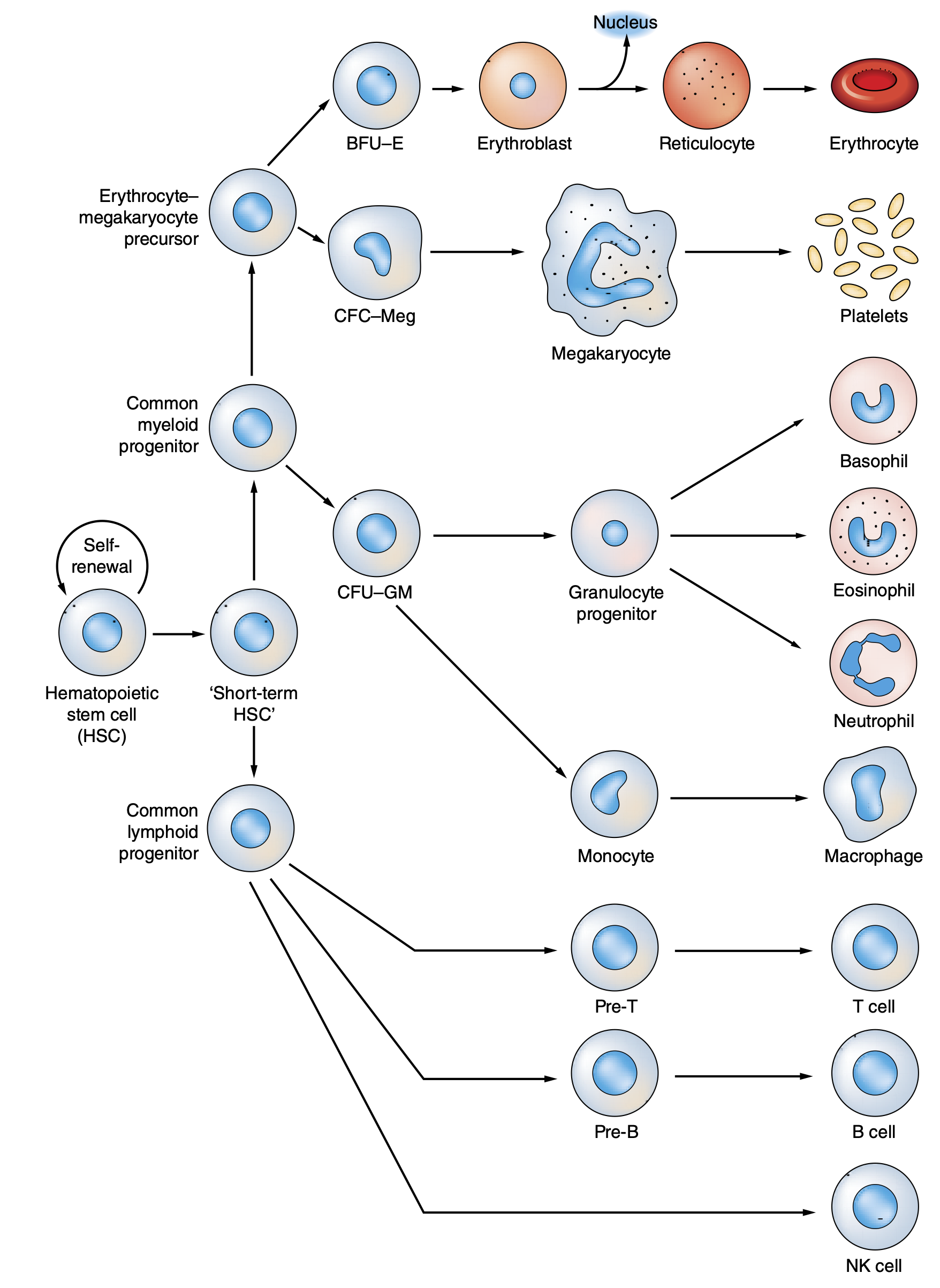
These cells are produced in the bone marrow and then move into the vascular so that they can move about the body and perform their functions (transport oxygen, clot, do adaptive and innate immune things).

Peripheral blood mononuclear cells (PBMCs)¶

It is possible to enrich for what are called PBMCs from vein by subjecting sample to density gradient centrifugation. This enrichs for cells that have one, round nucleus, and excludes cells that do not have nuclie, or that have multi-lobed structures. PBMCs typically contain:

... several classes of immune cells, including T cells (~70%), B cells (~15%), monocytes (~5%), dendritic cells (~1%) and natural killer (NK) cells (~10%)
-- Sen et al 2019

and

... The CD3+ lymphocytes are composed of CD4+ and CD8+ T cells, roughly in a 2:1 ratio.
-- Kleiveland, 2015

Bio question(s) for the day¶

• What does scRNAseq estimate as their relative proportion? and how does it compare to the estimate above?
• To what extent does cell type composition vary between samples?
• Are there other genes that are better at distinguishing between these populations than marker genes listed below?
• How many cells do you need to reliably detect a sub-population?

Data¶

10X Genomics scRNA-seq on human PBMCs

Sample 1¶

• http://cf.10xgenomics.com/samples/cell-exp/1.1.0/pbmc3k/pbmc3k_filtered_gene_bc_matrices.tar.gz

Sample 2¶

• https://colab.research.google.com/corgiredirector?site=https%3A%2F%2Fcf.10xgenomics.com%2Fsamples%2Fcell-exp%2F6.1.0%2F20k_PBMC_3p_HT_nextgem_Chromium_X%2F20k_PBMC_3p_HT_nextgem_Chromium_X_filtered_feature_bc_matrix.h5
• 20k Human PBMCs, 3’ HT v3.1, Chromium X
• Sourced from a healthy female donor
• 23,837 cells
• 35,000 reads per cell
• Filtered data in .h5 format

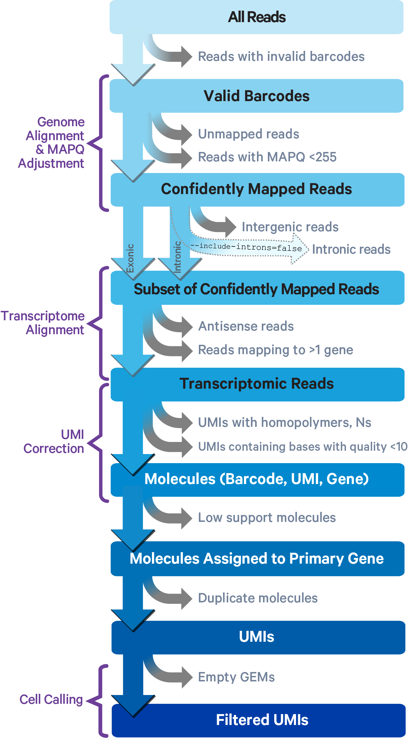
CellRanger¶

CellRanger is the program that converts sequencing reads into gene expression counts.

CellRanger flow chart from 10X genomics

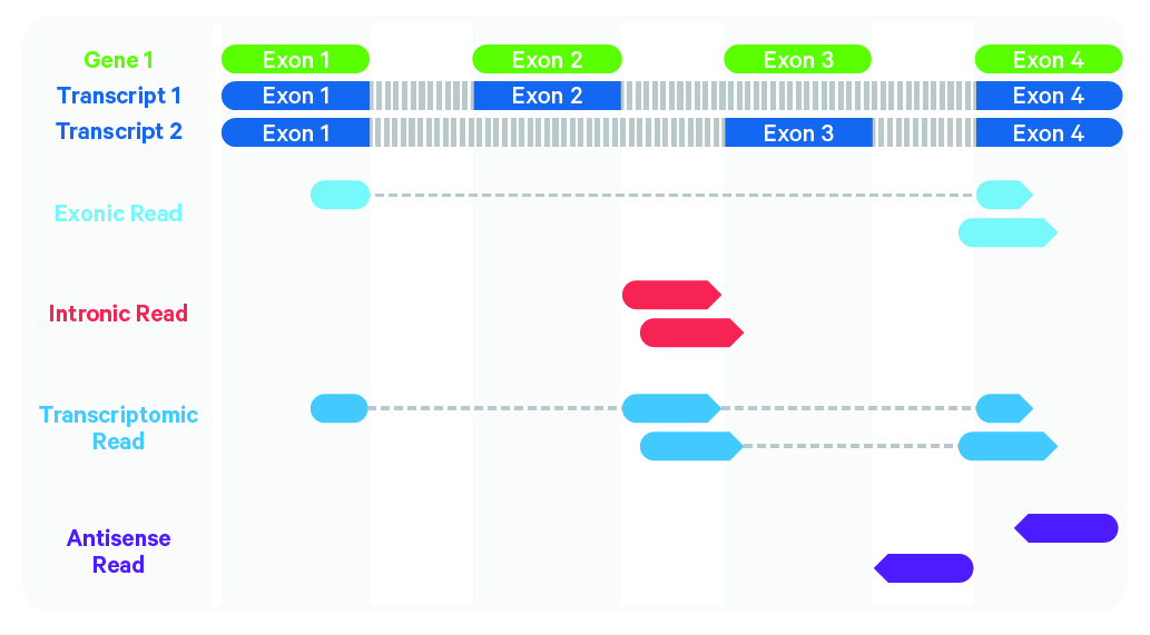
Here is a more detailed glimpse of what is happening here:

CellRanger flow chart 2 from 10X genomics

CellRanger mapping from 10X genomics

Installation¶

If you choose to analyze data from your own computer, please use an environment manager like conda.

In [1]:

# !pip install scanpy scipy umap-learn leidenalg

# !pip install scanpy scipy umap-learn leidenalg

Fetch data file(s)¶

In [2]:

# wget for linux/unix
# !wget https://cf.10xgenomics.com/samples/cell-exp/3.0.0/pbmc_10k_v3/pbmc_10k_v3_filtered_feature_bc_matrix.h5
# !wget https://cf.10xgenomics.com/samples/cell-exp/6.1.0/20k_PBMC_3p_HT_nextgem_Chromium_X/20k_PBMC_3p_HT_nextgem_Chromium_X_filtered_feature_bc_matrix.h5

# curl for macOS; i have no clue what to use for Windows
# !curl https://cf.10xgenomics.com/samples/cell-exp/3.0.0/pbmc_10k_v3/pbmc_10k_v3_filtered_feature_bc_matrix.h5 -o pbmc_10k_v3_filtered_feature_bc_matrix.h5
# !curl https://cf.10xgenomics.com/samples/cell-exp/6.1.0/20k_PBMC_3p_HT_nextgem_Chromium_X/20k_PBMC_3p_HT_nextgem_Chromium_X_filtered_feature_bc_matrix.h5 -o 20k_PBMC_3p_HT_nextgem_Chromium_X_filtered_feature_bc_matrix.h5

# wget for linux/unix # !wget https://cf.10xgenomics.com/samples/cell-exp/3.0.0/pbmc_10k_v3/pbmc_10k_v3_filtered_feature_bc_matrix.h5 # !wget https://cf.10xgenomics.com/samples/cell-exp/6.1.0/20k_PBMC_3p_HT_nextgem_Chromium_X/20k_PBMC_3p_HT_nextgem_Chromium_X_filtered_feature_bc_matrix.h5 # curl for macOS; i have no clue what to use for Windows # !curl https://cf.10xgenomics.com/samples/cell-exp/3.0.0/pbmc_10k_v3/pbmc_10k_v3_filtered_feature_bc_matrix.h5 -o pbmc_10k_v3_filtered_feature_bc_matrix.h5 # !curl https://cf.10xgenomics.com/samples/cell-exp/6.1.0/20k_PBMC_3p_HT_nextgem_Chromium_X/20k_PBMC_3p_HT_nextgem_Chromium_X_filtered_feature_bc_matrix.h5 -o 20k_PBMC_3p_HT_nextgem_Chromium_X_filtered_feature_bc_matrix.h5

Scanpy basics¶

load packages¶

In [3]:

import scanpy as sc
import numpy as np
import pandas as pd
import matplotlib.pyplot as plt
import warnings
# warnings.filterwarnings('ignore')
plt.rcParams['figure.dpi'] = 300
sc.logging.print_header()

import scanpy as sc import numpy as np import pandas as pd import matplotlib.pyplot as plt import warnings # warnings.filterwarnings('ignore') plt.rcParams['figure.dpi'] = 300 sc.logging.print_header()

/opt/homebrew/Caskroom/miniforge/base/envs/scnpy/lib/python3.12/site-packages/tqdm/auto.py:21: TqdmWarning: IProgress not found. Please update jupyter and ipywidgets. See https://ipywidgets.readthedocs.io/en/stable/user_install.html
  from .autonotebook import tqdm as notebook_tqdm

scanpy==1.10.4 anndata==0.11.3 umap==0.5.7 numpy==1.26.4 scipy==1.14.1 pandas==2.2.3 scikit-learn==1.6.1 statsmodels==0.14.4 igraph==0.11.8 pynndescent==0.5.13

Load Sample 1¶

In [4]:

# I have stored these data files in another dir
ad10f = sc.read_10x_h5("data/pbmc_10k_v3_filtered_feature_bc_matrix.h5")
# If you stored yours in the cwd on Colab, you should uncomment and run this line instead to load your data:
# ad10f = sc.read_10x_h5("pbmc_10k_v3_filtered_feature_bc_matrix.h5")

# I have stored these data files in another dir ad10f = sc.read_10x_h5("data/pbmc_10k_v3_filtered_feature_bc_matrix.h5") # If you stored yours in the cwd on Colab, you should uncomment and run this line instead to load your data: # ad10f = sc.read_10x_h5("pbmc_10k_v3_filtered_feature_bc_matrix.h5")

/opt/homebrew/Caskroom/miniforge/base/envs/scnpy/lib/python3.12/site-packages/anndata/_core/anndata.py:1758: UserWarning: Variable names are not unique. To make them unique, call `.var_names_make_unique`.
  utils.warn_names_duplicates("var")
/opt/homebrew/Caskroom/miniforge/base/envs/scnpy/lib/python3.12/site-packages/anndata/_core/anndata.py:1758: UserWarning: Variable names are not unique. To make them unique, call `.var_names_make_unique`.
  utils.warn_names_duplicates("var")

Getting information about functions¶

You can get info about functions using

help(functionName)

or

?functionName

Inspecting the data -- gross properties¶

In [5]:

ad10f.var_names_make_unique()

#?sc.read_10x_h5

ad10f.var_names_make_unique() #?sc.read_10x_h5

Package documentation¶

Often, the best source of help is the package's documentation.

Scanpy's documentation

In [6]:

print(ad10f)

print(ad10f)

AnnData object with n_obs × n_vars = 11769 × 33538
    var: 'gene_ids', 'feature_types', 'genome'

In [7]:

ad10f.shape

ad10f.shape

Out[7]:

(11769, 33538)

In [8]:

type(ad10f)

type(ad10f)

Out[8]:

anndata._core.anndata.AnnData

AnnData¶

AnnData is a Python package that defines a data structure designed to efficiently store large data sets like scRNA-seq.

AnnData schema. AnnData documentation. See Resouces below for more

Slicing or subsetting¶

There are lots of ways to get parts of an adata obkect. Here, let's randomly select a subset of cells and genes.

In [9]:

ncells = 3
ngenes = 4
randGenes = np.random.choice(ad10f.var_names, size=ngenes, replace=False)
randCells = np.random.choice(ad10f.obs_names, size=ncells, replace=False)

ncells = 3 ngenes = 4 randGenes = np.random.choice(ad10f.var_names, size=ngenes, replace=False) randCells = np.random.choice(ad10f.obs_names, size=ncells, replace=False)

In [10]:

print(randCells)

print(randCells)

['TTCCACGCAGACGATG-1' 'CATTGCCAGGTACAAT-1' 'ACTTTCAGTTGAGAGC-1']

In [11]:

print(randGenes)

print(randGenes)

['AC130352.1' 'AC092354.2' 'MOAP1' 'POLR3B']

In [12]:

newAnndata = ad10f[ randCells ]
newAnndata

newAnndata = ad10f[ randCells ] newAnndata

Out[12]:

View of AnnData object with n_obs × n_vars = 3 × 33538
    var: 'gene_ids', 'feature_types', 'genome'

In [13]:

ad10f[ randGenes ]

ad10f[ randGenes ]

---------------------------------------------------------------------------
KeyError                                  Traceback (most recent call last)
Cell In[13], line 1
----> 1 ad10f[ randGenes ]

File /opt/homebrew/Caskroom/miniforge/base/envs/scnpy/lib/python3.12/site-packages/anndata/_core/anndata.py:1022, in AnnData.__getitem__(self, index)
   1020 def __getitem__(self, index: Index) -> AnnData:
   1021     """Returns a sliced view of the object."""
-> 1022     oidx, vidx = self._normalize_indices(index)
   1023     return AnnData(self, oidx=oidx, vidx=vidx, asview=True)

File /opt/homebrew/Caskroom/miniforge/base/envs/scnpy/lib/python3.12/site-packages/anndata/_core/anndata.py:1003, in AnnData._normalize_indices(self, index)
   1002 def _normalize_indices(self, index: Index | None) -> tuple[slice, slice]:
-> 1003     return _normalize_indices(index, self.obs_names, self.var_names)

File /opt/homebrew/Caskroom/miniforge/base/envs/scnpy/lib/python3.12/site-packages/anndata/_core/index.py:32, in _normalize_indices(index, names0, names1)
     30     index = tuple(i.values if isinstance(i, pd.Series) else i for i in index)
     31 ax0, ax1 = unpack_index(index)
---> 32 ax0 = _normalize_index(ax0, names0)
     33 ax1 = _normalize_index(ax1, names1)
     34 return ax0, ax1

File /opt/homebrew/Caskroom/miniforge/base/envs/scnpy/lib/python3.12/site-packages/anndata/_core/index.py:105, in _normalize_index(indexer, index)
    103         if np.any(positions < 0):
    104             not_found = indexer[positions < 0]
--> 105             raise KeyError(
    106                 f"Values {list(not_found)}, from {list(indexer)}, "
    107                 "are not valid obs/ var names or indices."
    108             )
    109         return positions  # np.ndarray[int]
    110 raise IndexError(f"Unknown indexer {indexer!r} of type {type(indexer)}")

KeyError: "Values ['AC130352.1', 'AC092354.2', 'MOAP1', 'POLR3B'], from ['AC130352.1', 'AC092354.2', 'MOAP1', 'POLR3B'], are not valid obs/ var names or indices."

In [14]:

ad10f[:, randGenes ]

ad10f[:, randGenes ]

Out[14]:

View of AnnData object with n_obs × n_vars = 11769 × 4
    var: 'gene_ids', 'feature_types', 'genome'

In [15]:

gname_counts = ad10f.var_names.value_counts()
print(gname_counts)
np.any(gname_counts>1)

gname_counts = ad10f.var_names.value_counts() print(gname_counts) np.any(gname_counts>1)

MIR1302-2HG    1
DCT            1
GPC6-AS2       1
GPC6           1
AL354811.1     1
              ..
ORC3           1
RARS2          1
SLC35A1        1
AL049697.1     1
FAM231C        1
Name: count, Length: 33538, dtype: int64

Out[15]:

False

In [16]:

duplicates = gname_counts[gname_counts > 1]
print(duplicates)

duplicates = gname_counts[gname_counts > 1] print(duplicates)

Series([], Name: count, dtype: int64)

In [17]:

ad10f.var_names_make_unique()
ad10f[:, randGenes ]

ad10f.var_names_make_unique() ad10f[:, randGenes ]

Out[17]:

View of AnnData object with n_obs × n_vars = 11769 × 4
    var: 'gene_ids', 'feature_types', 'genome'

In [18]:

ad10f[randCells, randGenes ]

ad10f[randCells, randGenes ]

Out[18]:

View of AnnData object with n_obs × n_vars = 3 × 4
    var: 'gene_ids', 'feature_types', 'genome'

Views
Views are pointers to memory where original anndata is stored. They are not copies of the variable.

Gene counts¶

So, where is the data?

In [19]:

ad10f[randCells, randGenes ].X

ad10f[randCells, randGenes ].X

Out[19]:

<Compressed Sparse Row sparse matrix of dtype 'float32'
	with 1 stored elements and shape (3, 4)>

The Metadata¶

• for cells, see .obs
• for genesm see .var

In [20]:

print(ad10f.obs.columns)

print(ad10f.obs.columns)

Index([], dtype='object')

In [21]:

ad10f.obs['sample_name'] = "sample_1"
print(ad10f.obs.columns)

ad10f.obs['sample_name'] = "sample_1" print(ad10f.obs.columns)

Index(['sample_name'], dtype='object')

In [22]:

print(ad10f[randCells].obs)

print(ad10f[randCells].obs)

                   sample_name
TTCCACGCAGACGATG-1    sample_1
CATTGCCAGGTACAAT-1    sample_1
ACTTTCAGTTGAGAGC-1    sample_1

In [23]:

print(ad10f.var.columns)

print(ad10f.var.columns)

Index(['gene_ids', 'feature_types', 'genome'], dtype='object')

In [24]:

print(ad10f[:,randGenes].var)

print(ad10f[:,randGenes].var)

                   gene_ids    feature_types  genome
AC130352.1  ENSG00000270154  Gene Expression  GRCh38
AC092354.2  ENSG00000272370  Gene Expression  GRCh38
MOAP1       ENSG00000165943  Gene Expression  GRCh38
POLR3B      ENSG00000013503  Gene Expression  GRCh38

.loc¶

.obs and .var are Pandas dataframes and so you can access subsets of them using .loc and .iloc

In [25]:

print(ad10f.var.loc[randGenes])

print(ad10f.var.loc[randGenes])

                   gene_ids    feature_types  genome
AC130352.1  ENSG00000270154  Gene Expression  GRCh38
AC092354.2  ENSG00000272370  Gene Expression  GRCh38
MOAP1       ENSG00000165943  Gene Expression  GRCh38
POLR3B      ENSG00000013503  Gene Expression  GRCh38

Quality Control (QC)¶

Broadly speaking there are two things that we apply quality control to:

1. Cells: We want to find putative doublets and low quality cell barcodes and hold them out of downstram analysis.
2. Genes: We also can remove genes that are not detected in vast majority of cell

The function sc.pp.calculate_qc_metrics() will calculate a set of metrics on adata and place the results in .obs or .var. The results can then be used to filter the adata. pp.calculate_qc_metrics() can also take inputs to specify other, custom metrics to compute.

Below, we use it to compute the fraction of all UMIs in each cell that are mitochondrially encoded or that encode for ribosomal genes.

In [26]:

ad10f.var['mt'] = ad10f.var_names.str.startswith('MT-')
ribo_prefix = ("RPS","RPL")
ad10f.var['ribo'] = ad10f.var_names.str.startswith(ribo_prefix)
sc.pp.calculate_qc_metrics(ad10f, qc_vars=['mt','ribo'], percent_top=None, log1p=False, inplace=True)

ad10f.var['mt'] = ad10f.var_names.str.startswith('MT-') ribo_prefix = ("RPS","RPL") ad10f.var['ribo'] = ad10f.var_names.str.startswith(ribo_prefix) sc.pp.calculate_qc_metrics(ad10f, qc_vars=['mt','ribo'], percent_top=None, log1p=False, inplace=True)

Visualize¶

Take a look some typical QC values across these data

In [27]:

adClean = ad10f.copy()

fig, (ax1, ax2, ax3) = plt.subplots(1, 3, figsize=(10,4), gridspec_kw={'wspace':0.25}, constrained_layout=True)
ax1_dict = sc.pl.scatter(adClean, x='total_counts', y='pct_counts_mt', ax=ax1, show=False)
ax2_dict = sc.pl.scatter(adClean, x='total_counts', y='n_genes_by_counts',ax=ax2, show=False)
ax3_dict = sc.pl.scatter(adClean, x='pct_counts_ribo', y='n_genes_by_counts',ax=ax3, show=False)
plt.show()

adClean = ad10f.copy() fig, (ax1, ax2, ax3) = plt.subplots(1, 3, figsize=(10,4), gridspec_kw={'wspace':0.25}, constrained_layout=True) ax1_dict = sc.pl.scatter(adClean, x='total_counts', y='pct_counts_mt', ax=ax1, show=False) ax2_dict = sc.pl.scatter(adClean, x='total_counts', y='n_genes_by_counts',ax=ax2, show=False) ax3_dict = sc.pl.scatter(adClean, x='pct_counts_ribo', y='n_genes_by_counts',ax=ax3, show=False) plt.show()

Now, do the filtering.

First, keep cells with fewer than 20% mitochondrially encoded gene total UMIs

In [28]:

adClean = adClean[adClean.obs['pct_counts_mt']<20,:].copy()
adClean.n_obs

adClean = adClean[adClean.obs['pct_counts_mt']<20,:].copy() adClean.n_obs

Out[28]:

11047

Second, filter based on total number of genes detected (at least 500). Third, filter based on total number of counts (fewer than than 30,000) Fourth, keep genes that are detected in at least 3 cells.

In [29]:

sc.pp.filter_cells(adClean, min_genes=500)
print(adClean.n_obs)

sc.pp.filter_cells(adClean, max_counts=30000)
print(adClean.n_obs)

sc.pp.filter_genes(adClean, min_cells=3)
print(adClean.shape)

sc.pp.filter_cells(adClean, min_genes=500) print(adClean.n_obs) sc.pp.filter_cells(adClean, max_counts=30000) print(adClean.n_obs) sc.pp.filter_genes(adClean, min_cells=3) print(adClean.shape)

10924
10891
(10891, 20181)

Normalization¶

Simple library size scaling, then log transform. There are many other ways to correct for cell-to-cell technical variation, for example different cell lysis efficiencies, but this method is good enough for this data set and our goals.

In [30]:

adNorm = adClean.copy()
adNorm.layers['counts'] = adNorm.X.copy()
sc.pp.normalize_total(adNorm , target_sum=1e4)
sc.pp.log1p(adNorm)
adNorm.layers['lognorm'] = adNorm.X.copy()

adNorm = adClean.copy() adNorm.layers['counts'] = adNorm.X.copy() sc.pp.normalize_total(adNorm , target_sum=1e4) sc.pp.log1p(adNorm) adNorm.layers['lognorm'] = adNorm.X.copy()

Highly variable genes (HVG)¶

It is common practice to limit some parts of analysis to those variables/genes that exhibit some degree of variation in their values across the data. We call these highly variable genes, or HVG for short. To find these, calculate some gene statistics, which when combined with thresholds below, determine which genes are considered HVG. The relevant metrics are:

1. mean expression
2. dispersion, which is the variance / mean.

Variance is defined as the expected squared deviation of gene expression. The normalized dispersion is calculated by scaling based on a bin of mean expression.

In [31]:

sc.pp.highly_variable_genes(adNorm , min_mean=0.0125, max_mean=6, min_disp=0.25)
adNorm.var

sc.pp.highly_variable_genes(adNorm , min_mean=0.0125, max_mean=6, min_disp=0.25) adNorm.var

Out[31]:

	gene_ids	feature_types	genome	mt	ribo	n_cells_by_counts	mean_counts	pct_dropout_by_counts	total_counts	n_cells	highly_variable	means	dispersions	dispersions_norm
AL627309.1	ENSG00000238009	Gene Expression	GRCh38	False	False	60	0.005183	99.490186	61.0	60	False	0.007519	0.595591	-0.001919
AL627309.3	ENSG00000239945	Gene Expression	GRCh38	False	False	4	0.000340	99.966012	4.0	4	False	0.000389	0.144284	-1.366927
AL669831.5	ENSG00000237491	Gene Expression	GRCh38	False	False	679	0.062367	94.230606	734.0	665	False	0.077585	0.586329	-0.029932
FAM87B	ENSG00000177757	Gene Expression	GRCh38	False	False	13	0.001190	99.889540	14.0	13	False	0.001139	0.169543	-1.290532
LINC00115	ENSG00000225880	Gene Expression	GRCh38	False	False	350	0.031269	97.026085	368.0	337	False	0.038579	0.459107	-0.414723
...	...	...	...	...	...	...	...	...	...	...	...	...	...	...
AC011043.1	ENSG00000276256	Gene Expression	GRCh38	False	False	77	0.006882	99.345739	81.0	74	False	0.010262	0.738345	0.429851
AL592183.1	ENSG00000273748	Gene Expression	GRCh38	False	False	32	0.002719	99.728099	32.0	30	False	0.003977	0.799225	0.613985
AC007325.4	ENSG00000278817	Gene Expression	GRCh38	False	False	239	0.020902	97.969241	246.0	233	False	0.023936	0.329110	-0.807909
AL354822.1	ENSG00000278384	Gene Expression	GRCh38	False	False	319	0.028210	97.289489	332.0	303	False	0.038089	0.594378	-0.005588
AC240274.1	ENSG00000271254	Gene Expression	GRCh38	False	False	101	0.008752	99.141813	103.0	99	False	0.010213	0.301150	-0.892475

20181 rows × 14 columns

In [32]:

sc.pl.highly_variable_genes(adNorm)

sc.pl.highly_variable_genes(adNorm)

Dimensionality reduction with Principal components analysis (PCA)¶

Why performan dimentaionality reduction?

1. Genes are expressed in coordinated fashion, meaning that many have correlated expression patterns and so PCA reduces the computational complexity of downstream analysis
2. scRNA-seq data is noisy on a per gene basis.

PCA allows us to reduce a high dimensional data set into a lower dimension in which much of the total variation is maintained. To understand PCA, you need to know linear algebra. In essence, it identifies sets of linear combinations of genes in such a way that a PC is uncorrelated with other PCs and that explains most variation in the data. The function call sc.tl.pca does the following:

1. computes the covariance matrix (correlation between each pair of genes)
2. finds eigenvectors (directions of axes that maximize that variance), orthogonal to each other

Later, we select a threshold (n_pcs) as the number of PCs that contribute most to the total variation on our data. We use these n_pcs PCs to compute cell-to-cell distances for embedding (2D visualization via UMAP) and for clustering of cells.

In [33]:

sc.tl.pca(adNorm , mask_var='highly_variable')

sc.tl.pca(adNorm , mask_var='highly_variable')

Marker genes¶

Here PBMC cell types and some genes that have been used to identify them:
Monocytes: CD14, CD68, LYZ
Dendritic: CLEC4C, FLT3
NK cells: GNLY, NCAM1
B cells: CD19, CD79A, CD79B
T cells: CD3D, CD3E, TRAC, TRBC

In [34]:

markerGenes = ['CD14','CLEC4C', 'CD19',  'GNLY', 'CD3D']
sc.pl.pca(adNorm , color=markerGenes, ncols=2, layer='counts')

markerGenes = ['CD14','CLEC4C', 'CD19', 'GNLY', 'CD3D'] sc.pl.pca(adNorm , color=markerGenes, ncols=2, layer='counts')

In [35]:

sc.pl.pca(adNorm , color=markerGenes, ncols=2)

sc.pl.pca(adNorm , color=markerGenes, ncols=2)

In [36]:

sc.pl.pca(adNorm, color=['total_counts', 'pct_counts_mt', 'pct_counts_ribo'], s=25,ncols=3)

sc.pl.pca(adNorm, color=['total_counts', 'pct_counts_mt', 'pct_counts_ribo'], s=25,ncols=3)

In [37]:

sc.pl.pca_variance_ratio(adNorm, 50)

sc.pl.pca_variance_ratio(adNorm, 50)

PCA Loadings¶

Where are PCs (i.e. loadings -- the contribution of each gene to each PC) stored in anndata? .varm (see figure of anndata way above)?

In [38]:

np.shape(adNorm.varm["PCs"])

np.shape(adNorm.varm["PCs"])

Out[38]:

(20181, 50)

Where are the PC values of each cell (i.e. the PC scores) stored in anndata? .obsm

In [39]:

np.shape(adNorm.obsm["X_pca"])

np.shape(adNorm.obsm["X_pca"])

Out[39]:

(10891, 50)

kNN cell-cell distances¶

The k-nearest neighbor graph generates an adjacency matrix by finding, for each cell, the k cells that are closest to it. This helps to reduce noise in computing cell-cell distances or similarities and is important for embedding the cells in a 2D space, and for community detection algorithms. Two arguments are n_neighbors, or k, and the number of PCs to use when computing cell-cell distances.

In [40]:

n_neighbors = 20
n_pcs = 10
sc.pp.neighbors(adNorm, n_neighbors=n_neighbors, n_pcs=n_pcs)

n_neighbors = 20 n_pcs = 10 sc.pp.neighbors(adNorm, n_neighbors=n_neighbors, n_pcs=n_pcs)

Visualization of cell-cell similarities¶

UMAP embedding¶

This an elaboration on the t-SNE embedding approach. Both of these methods try to project cells into a reduced (typically 2) dimensional coordinate system while maintaining both the global and local structure of the high dimensional space of the data (i.e. cells that are distant from each other high dimensions should still be distant in the reduced embedding; same is true for cells that are near each other). The distances come from the kNN graph.

In [41]:

sc.tl.umap(adNorm, 0.25)

sc.tl.umap(adNorm, 0.25)

/var/folders/1_/v5grqr5n7kj42276bb6ryxj00000gn/T/ipykernel_66578/2021512077.py:1: FutureWarning: The specified parameters ('min_dist',) are no longer positional. Please specify them like `min_dist=0.25`
  sc.tl.umap(adNorm, 0.25)

In [42]:

sc.pl.umap(adNorm, color=markerGenes, alpha=.75, s=15, ncols=2)

sc.pl.umap(adNorm, color=markerGenes, alpha=.75, s=15, ncols=2)

Unsupervised clustering¶

Let's try to assign cells to distinct groups or clusters based on the cell-to-cell distances. Leiden and Louvain are examples of community detection methods that perform this task by searching for the group assignment that maximize within group similarity (which is equivalent to within group edges of a knn graph) and to minimize between group similarity.

In [43]:

sc.tl.leiden(adNorm,.1)

sc.tl.leiden(adNorm,.1)

/var/folders/1_/v5grqr5n7kj42276bb6ryxj00000gn/T/ipykernel_66578/3992796732.py:1: FutureWarning: In the future, the default backend for leiden will be igraph instead of leidenalg.

 To achieve the future defaults please pass: flavor="igraph" and n_iterations=2.  directed must also be False to work with igraph's implementation.
  sc.tl.leiden(adNorm,.1)

In [44]:

sc.pl.umap(adNorm,color=['leiden'], alpha=.75, s=15, legend_loc='on data')

sc.pl.umap(adNorm,color=['leiden'], alpha=.75, s=15, legend_loc='on data')

Discordance
Embeddings do not always agree with cluster results! See cluster 2 above.

We can try to rectify this by using PAGA, which tries to infer dynamic relationships between clusters, to seed an initial embedding for UMAP that reflects overall cluster similarities.

In the next cell, we call the following functions

tl.paga() computes intercluster similarities

pl.paga() creates an intial embedding based on this

tl.umap() uses this embedding to start its optimization

Let's restart with the cleaned data.

In [45]:

adNorm = adClean.copy()

## Norm, HVG, PCA, kNN
sc.pp.normalize_total(adNorm , target_sum=1e4)
sc.pp.log1p(adNorm)
sc.pp.highly_variable_genes(adNorm , min_mean=0.0125, max_mean=6, min_disp=0.25)
sc.tl.pca(adNorm , use_highly_variable=True)

n_neighbors = 20
n_pcs = 10
sc.pp.neighbors(adNorm, n_neighbors=n_neighbors, n_pcs=n_pcs)
sc.tl.leiden(adNorm,.1)
sc.tl.paga(adNorm)
sc.pl.paga(adNorm, plot=False)
sc.tl.umap(adNorm, 0.25, init_pos='paga')
sc.pl.umap(adNorm,color=['leiden'], alpha=.75, s=15, legend_loc='on data')

adNorm = adClean.copy() ## Norm, HVG, PCA, kNN sc.pp.normalize_total(adNorm , target_sum=1e4) sc.pp.log1p(adNorm) sc.pp.highly_variable_genes(adNorm , min_mean=0.0125, max_mean=6, min_disp=0.25) sc.tl.pca(adNorm , use_highly_variable=True) n_neighbors = 20 n_pcs = 10 sc.pp.neighbors(adNorm, n_neighbors=n_neighbors, n_pcs=n_pcs) sc.tl.leiden(adNorm,.1) sc.tl.paga(adNorm) sc.pl.paga(adNorm, plot=False) sc.tl.umap(adNorm, 0.25, init_pos='paga') sc.pl.umap(adNorm,color=['leiden'], alpha=.75, s=15, legend_loc='on data')

/opt/homebrew/Caskroom/miniforge/base/envs/scnpy/lib/python3.12/site-packages/scanpy/preprocessing/_pca.py:374: FutureWarning: Argument `use_highly_variable` is deprecated, consider using the mask argument. Use_highly_variable=True can be called through mask_var="highly_variable". Use_highly_variable=False can be called through mask_var=None
  warn(msg, FutureWarning)
/var/folders/1_/v5grqr5n7kj42276bb6ryxj00000gn/T/ipykernel_66578/3419511010.py:15: FutureWarning: The specified parameters ('min_dist',) are no longer positional. Please specify them like `min_dist=0.25`
  sc.tl.umap(adNorm, 0.25, init_pos='paga')

In [46]:

sc.pl.umap(adNorm , color=markerGenes, ncols=2)

sc.pl.umap(adNorm , color=markerGenes, ncols=2)

Make a figure that shows the embedding and expression of marker genes side-by-side. Note that I am adding markers for T cell, B cell, and Monocyte sub-types

In [47]:

marker_genes_broad_dict = {
    'B cell': ['CD79A', 'PAX5'],
    'Dendritic': ['CLEC4C', 'FCER1A'],
    'Monocyte': ['CSF1R', 'FCGR3A'],
    'NK cell': ['NKG7', 'GNLY'],
    'T cell': ['TRAC', 'CD3E'],
}

fig, (ax1, ax2) = plt.subplots(1, 2, figsize=(10,4), gridspec_kw={'wspace':0.25})
ax1_dict = sc.pl.umap(adNorm,color=['leiden'], alpha=.75, s=10, legend_loc='on data', ax=ax1, show=False)
ax2_dict = sc.pl.dotplot(adNorm, marker_genes_broad_dict, 'leiden', dendrogram=True,ax=ax2, show=False)
plt.show()

marker_genes_broad_dict = { 'B cell': ['CD79A', 'PAX5'], 'Dendritic': ['CLEC4C', 'FCER1A'], 'Monocyte': ['CSF1R', 'FCGR3A'], 'NK cell': ['NKG7', 'GNLY'], 'T cell': ['TRAC', 'CD3E'], } fig, (ax1, ax2) = plt.subplots(1, 2, figsize=(10,4), gridspec_kw={'wspace':0.25}) ax1_dict = sc.pl.umap(adNorm,color=['leiden'], alpha=.75, s=10, legend_loc='on data', ax=ax1, show=False) ax2_dict = sc.pl.dotplot(adNorm, marker_genes_broad_dict, 'leiden', dendrogram=True,ax=ax2, show=False) plt.show()

WARNING: dendrogram data not found (using key=dendrogram_leiden). Running `sc.tl.dendrogram` with default parameters. For fine tuning it is recommended to run `sc.tl.dendrogram` independently.
WARNING: Groups are not reordered because the `groupby` categories and the `var_group_labels` are different.
categories: 0, 1, 2, etc.
var_group_labels: B cell, Dendritic, Monocyte, etc.

Cluster annotation¶

We can walk down the rows of the dotplot and guess at the cell types of some of these clusters based on the specificty of marker expression:

cluster	markers of	cell type
5	B, Dendritic, Mono	???
1	Monocyte	Monocyte
4	Monocyte, T	???
3	B	B-cell
6	Dendritic (B/Mono?)	Dendritic cell
7	none	Mystery cell
0	T cell	T cell
2	NK/T	???

Some clusters are ambiguous because they express markers of more than one cell type. This could be due to the cluster containing > 1 cell type, or because the cell barcodes are doublets. If the former, then we should be able to sub cluster them. Let's try this.

Clusters to refine are 5, 4, and 2.

In [48]:

sc.tl.leiden(adNorm,.1, restrict_to=["leiden",["5"]])
sc.tl.dendrogram(adNorm, "leiden_R")
fig, (ax1, ax2) = plt.subplots(1, 2, figsize=(10,4), gridspec_kw={'wspace':0.25})
ax1_dict = sc.pl.umap(adNorm,color=['leiden_R'], alpha=.75, s=10, legend_loc='on data', ax=ax1, show=False)
ax2_dict = sc.pl.dotplot(adNorm, marker_genes_broad_dict, 'leiden_R', dendrogram=True,ax=ax2, show=False)
plt.show()

sc.tl.leiden(adNorm,.1, restrict_to=["leiden",["5"]]) sc.tl.dendrogram(adNorm, "leiden_R") fig, (ax1, ax2) = plt.subplots(1, 2, figsize=(10,4), gridspec_kw={'wspace':0.25}) ax1_dict = sc.pl.umap(adNorm,color=['leiden_R'], alpha=.75, s=10, legend_loc='on data', ax=ax1, show=False) ax2_dict = sc.pl.dotplot(adNorm, marker_genes_broad_dict, 'leiden_R', dendrogram=True,ax=ax2, show=False) plt.show()

WARNING: Groups are not reordered because the `groupby` categories and the `var_group_labels` are different.
categories: 0, 1, 2, etc.
var_group_labels: B cell, Dendritic, Monocyte, etc.

Cluster 5 is split into 2 clusters now. Both of these sub-clusters express the Monocyte marker CD14, but are distinguished by their expression of dendritic marker FCER1A and the B cell genes CD79A and PAX5. Let's look at the QC metrics to see if that can give us additional hints as to whether these are real cells or are doublets.

In [49]:

sc.pl.violin(adNorm, ['total_counts'], groupby='leiden_R' )

sc.pl.violin(adNorm, ['total_counts'], groupby='leiden_R' )

Cluster 5 (and each sub-cluster) has a high number of Total counts. So let's annotate these as 'doublet'.

What about the other questionable clusters 4 and 2? Can we refine those?

In [50]:

# cluster 2 first
sc.tl.leiden(adNorm,.05, restrict_to=["leiden",["2"]])
sc.tl.dendrogram(adNorm, "leiden_R")
fig, (ax1, ax2) = plt.subplots(1, 2, figsize=(10,4), gridspec_kw={'wspace':0.25})
ax1_dict = sc.pl.umap(adNorm,color=['leiden_R'], alpha=.75, s=10, legend_loc='on data', ax=ax1, show=False)
ax2_dict = sc.pl.dotplot(adNorm, marker_genes_broad_dict, 'leiden_R', dendrogram=True,ax=ax2, show=False)
plt.show()

# cluster 2 first sc.tl.leiden(adNorm,.05, restrict_to=["leiden",["2"]]) sc.tl.dendrogram(adNorm, "leiden_R") fig, (ax1, ax2) = plt.subplots(1, 2, figsize=(10,4), gridspec_kw={'wspace':0.25}) ax1_dict = sc.pl.umap(adNorm,color=['leiden_R'], alpha=.75, s=10, legend_loc='on data', ax=ax1, show=False) ax2_dict = sc.pl.dotplot(adNorm, marker_genes_broad_dict, 'leiden_R', dendrogram=True,ax=ax2, show=False) plt.show()

WARNING: Groups are not reordered because the `groupby` categories and the `var_group_labels` are different.
categories: 0, 1, 2,0, etc.
var_group_labels: B cell, Dendritic, Monocyte, etc.

It looks like 2,0 is T cell, and 2,1 is Natural Killer cell. Note that 2,0 still has a distinct profile as compared to 0.

What about cluster 4? And this time, when we do the sub-clustering, let's keep the way that we split up cluster 2.

In [51]:

sc.tl.leiden(adNorm,.1, restrict_to=["leiden_R",["4"]])
sc.tl.dendrogram(adNorm, "leiden_R")
fig, (ax1, ax2) = plt.subplots(1, 2, figsize=(10,4), gridspec_kw={'wspace':0.25})
ax1_dict = sc.pl.umap(adNorm,color=['leiden_R'], alpha=.75, s=10, legend_loc='on data', ax=ax1, show=False)
ax2_dict = sc.pl.dotplot(adNorm, marker_genes_broad_dict, 'leiden_R', dendrogram=True,ax=ax2, show=False)
plt.show()

sc.tl.leiden(adNorm,.1, restrict_to=["leiden_R",["4"]]) sc.tl.dendrogram(adNorm, "leiden_R") fig, (ax1, ax2) = plt.subplots(1, 2, figsize=(10,4), gridspec_kw={'wspace':0.25}) ax1_dict = sc.pl.umap(adNorm,color=['leiden_R'], alpha=.75, s=10, legend_loc='on data', ax=ax1, show=False) ax2_dict = sc.pl.dotplot(adNorm, marker_genes_broad_dict, 'leiden_R', dendrogram=True,ax=ax2, show=False) plt.show()

WARNING: Groups are not reordered because the `groupby` categories and the `var_group_labels` are different.
categories: 0, 1, 2,0, etc.
var_group_labels: B cell, Dendritic, Monocyte, etc.

Is 4,1 multiplet?

In [52]:

sc.pl.violin(adNorm, ['total_counts', 'n_genes_by_counts'], groupby='leiden_R' )

sc.pl.violin(adNorm, ['total_counts', 'n_genes_by_counts'], groupby='leiden_R' )

Yes, it looks like 4,1 is similar in these QC profiles to cluster 5.

So our updated annotation table is now:

cluster	markers of	cell type
5	B, Dendritic, Mono	doublet
1	Monocyte	Monocyte
4,0	Monocyte	Monocyte
3	B	B-cell
6	Dendritic (B/Mono?)	Dendritic cell
7	none	Mystery cell
0	T cell	T cell
2,0	T cell	T cell
2,1	NK cell	NK cell

Why do we have two Monocyte clusters and two T cells clusters?

In [53]:

marker_genes_sub_dict = {
    'B cell': ['CD79A'],
    'Dendritic': ['CLEC4C'],
    'CD14 monocyte': ['CD14'],
    'CD16 monocyte': ['FCGR3A'],
    'NK cell': ['GNLY'],
    'CD4 T cell': ['CD4', 'GATA3'],
    'CD8 T cell': ['CD8A', 'EOMES']
}

fig, (ax1, ax2) = plt.subplots(1, 2, figsize=(10,4), gridspec_kw={'wspace':0.25})
ax1_dict = sc.pl.umap(adNorm,color=['leiden_R'], alpha=.75, s=10, legend_loc='on data', ax=ax1, show=False)
ax2_dict = sc.pl.dotplot(adNorm, marker_genes_sub_dict, 'leiden_R', dendrogram=True,ax=ax2, show=False)
plt.show()

marker_genes_sub_dict = { 'B cell': ['CD79A'], 'Dendritic': ['CLEC4C'], 'CD14 monocyte': ['CD14'], 'CD16 monocyte': ['FCGR3A'], 'NK cell': ['GNLY'], 'CD4 T cell': ['CD4', 'GATA3'], 'CD8 T cell': ['CD8A', 'EOMES'] } fig, (ax1, ax2) = plt.subplots(1, 2, figsize=(10,4), gridspec_kw={'wspace':0.25}) ax1_dict = sc.pl.umap(adNorm,color=['leiden_R'], alpha=.75, s=10, legend_loc='on data', ax=ax1, show=False) ax2_dict = sc.pl.dotplot(adNorm, marker_genes_sub_dict, 'leiden_R', dendrogram=True,ax=ax2, show=False) plt.show()

WARNING: Groups are not reordered because the `groupby` categories and the `var_group_labels` are different.
categories: 0, 1, 2,0, etc.
var_group_labels: B cell, Dendritic, CD14 monocyte, etc.

We are close to a final annotation now:

cluster	markers of	cell type
5	B, Dendritic, Mono	doublet
1	Monocyte	CD14 Monocyte
4,0	Monocyte	CD16 Monocyte
3	B	B-cell
6	Dendritic (B/Mono?)	Dendritic cell
7	none	Mystery cell
0	T cell	CD4 T cell
2,0	T cell	CD8 T cell
2,1	NK cell	NK cell

But what is cluster 7? It has low counts. If it is just ambient 'soup', then we would not expect it to have high levels of cell type specific genes. Let's do differential gene expression analysis to see what is upregulated in this cluster.

Differential gene expression¶

In [54]:

sc.tl.rank_genes_groups(adNorm, use_raw=False, groupby="leiden_R")

sc.tl.rank_genes_groups(adNorm, use_raw=False, groupby="leiden_R")

In [55]:

sc.pl.rank_genes_groups_dotplot(adNorm, n_genes=5, groupby="leiden_R", dendrogram=True, key='rank_genes_groups')

sc.pl.rank_genes_groups_dotplot(adNorm, n_genes=5, groupby="leiden_R", dendrogram=True, key='rank_genes_groups')

In [56]:

sc.pl.rank_genes_groups_dotplot(adNorm, n_genes=20, groupby="leiden_R", dendrogram=True, key='rank_genes_groups', groups=['7'])

sc.pl.rank_genes_groups_dotplot(adNorm, n_genes=20, groupby="leiden_R", dendrogram=True, key='rank_genes_groups', groups=['7'])

WARNING: Groups are not reordered because the `groupby` categories and the `var_group_labels` are different.
categories: 0, 1, 2,0, etc.
var_group_labels: 7

Although this result could be refined and explored a lot, it is sufficient for us to address our question about the identity of cluster 7 as follows:

Help from ChatGPT to annotate cells

Now, let's add the annotation to the anndata.obs and discard the other cells

cluster	markers of	cell type
1	Monocyte	CD14 Monocyte
4,0	Monocyte	CD16 Monocyte
3	B	B-cell
6	Dendritic (B/Mono?)	Dendritic cell
7	none	Platelet
0	T cell	CD4 T cell
2,0	T cell	CD8 T cell
2,1	NK cell	NK cell

In [57]:

tokeep = ["1", "4,0", "3", "6", "7", "0", "2,0", "2,1"]
adNorm2 = adNorm.copy()
adNorm2 = adNorm2[adNorm2.obs['leiden_R'].isin(tokeep)].copy()
adNorm2.shape
adNorm2.obs['leiden_R'].value_counts()

tokeep = ["1", "4,0", "3", "6", "7", "0", "2,0", "2,1"] adNorm2 = adNorm.copy() adNorm2 = adNorm2[adNorm2.obs['leiden_R'].isin(tokeep)].copy() adNorm2.shape adNorm2.obs['leiden_R'].value_counts()

Out[57]:

leiden_R
0      3563
1      3115
3      1604
2,0    1031
2,1     611
4,0     368
6        81
7        60
Name: count, dtype: int64

In [58]:

cell_dict = {'Dendritic': ['6'],
             'CD14 Monocyte': ['1'],
             'CD16 Monocyte': ["4,0"],
             'B cell': ['3'],
             'Platelet': ['7'],
             'CD4 T cell': ['0'],
             'CD8 T cell': ["2,0"],
             'NK cell': ["2,1"]
}

marker_genes_dict = {
    'B cell': ['CD79A'],
    'Dendritic': ['CLEC4C'],
    'CD14 monocyte': ['CD14'],
    'CD16 monocyte': ['FCGR3A'],
    'NK cell': ['GNLY'],
    'CD4 T cell': ['CD4', 'GATA3'],
    'CD8 T cell': ['CD8A', 'EOMES'],
    'Platelet': ['PF4', 'CAVIN2']
}


new_obs_name = 'cell_type'
adNorm2.obs[new_obs_name] = np.nan

for i in cell_dict.keys():
    ind = pd.Series(adNorm2.obs.leiden_R).isin(cell_dict[i])
    adNorm2.obs.loc[ind,new_obs_name] = i

adNorm2.obs['cell_type'] = adNorm2.obs['cell_type'].astype("category")

cell_dict = {'Dendritic': ['6'], 'CD14 Monocyte': ['1'], 'CD16 Monocyte': ["4,0"], 'B cell': ['3'], 'Platelet': ['7'], 'CD4 T cell': ['0'], 'CD8 T cell': ["2,0"], 'NK cell': ["2,1"] } marker_genes_dict = { 'B cell': ['CD79A'], 'Dendritic': ['CLEC4C'], 'CD14 monocyte': ['CD14'], 'CD16 monocyte': ['FCGR3A'], 'NK cell': ['GNLY'], 'CD4 T cell': ['CD4', 'GATA3'], 'CD8 T cell': ['CD8A', 'EOMES'], 'Platelet': ['PF4', 'CAVIN2'] } new_obs_name = 'cell_type' adNorm2.obs[new_obs_name] = np.nan for i in cell_dict.keys(): ind = pd.Series(adNorm2.obs.leiden_R).isin(cell_dict[i]) adNorm2.obs.loc[ind,new_obs_name] = i adNorm2.obs['cell_type'] = adNorm2.obs['cell_type'].astype("category")

/var/folders/1_/v5grqr5n7kj42276bb6ryxj00000gn/T/ipykernel_66578/4042500018.py:28: FutureWarning: Setting an item of incompatible dtype is deprecated and will raise an error in a future version of pandas. Value 'Dendritic' has dtype incompatible with float64, please explicitly cast to a compatible dtype first.
  adNorm2.obs.loc[ind,new_obs_name] = i

In [59]:

sc.tl.dendrogram(adNorm2, "cell_type")
fig, (ax1, ax2) = plt.subplots(1, 2, figsize=(12,5), gridspec_kw={'wspace':0.4})
ax1_dict = sc.pl.umap(adNorm2,color=['cell_type'], alpha=.75, s=10, legend_loc='on data', ax=ax1, show=False)
ax2_dict = sc.pl.dotplot(adNorm2, marker_genes_dict, 'cell_type', dendrogram=True,ax=ax2, show=False)
plt.show()

sc.tl.dendrogram(adNorm2, "cell_type") fig, (ax1, ax2) = plt.subplots(1, 2, figsize=(12,5), gridspec_kw={'wspace':0.4}) ax1_dict = sc.pl.umap(adNorm2,color=['cell_type'], alpha=.75, s=10, legend_loc='on data', ax=ax1, show=False) ax2_dict = sc.pl.dotplot(adNorm2, marker_genes_dict, 'cell_type', dendrogram=True,ax=ax2, show=False) plt.show()

WARNING: Groups are not reordered because the `groupby` categories and the `var_group_labels` are different.
categories: B cell, CD14 Monocyte, CD16 Monocyte, etc.
var_group_labels: B cell, Dendritic, CD14 monocyte, etc.

In [60]:

sc.pl.pca(adNorm2, color=['cell_type', 'GNLY'], alpha=.75, s=15, projection='3d')

sc.pl.pca(adNorm2, color=['cell_type', 'GNLY'], alpha=.75, s=15, projection='3d')

Differential expression analysis¶

Let's identify genes that are preferenntially expressed in each cluster versus all the others as a final step to annotate these clusters and to remove ones that are likely to be doublets.

In [61]:

sc.tl.rank_genes_groups(adNorm2, use_raw=False, groupby="cell_type")

sc.tl.rank_genes_groups(adNorm2, use_raw=False, groupby="cell_type")

Dot plot of differentially expressed genes¶

First, we will apply a filter so that we only display genes that meet additional criteria beyond statistical: fold change, % expressed in cluster, % expressed in other cells

In [62]:

sc.tl.filter_rank_genes_groups(adNorm2, min_fold_change=.7, min_in_group_fraction=.5, max_out_group_fraction=.15)
sc.pl.rank_genes_groups_dotplot(adNorm2, n_genes=6, groupby="cell_type", dendrogram=True, key='rank_genes_groups_filtered')

sc.tl.filter_rank_genes_groups(adNorm2, min_fold_change=.7, min_in_group_fraction=.5, max_out_group_fraction=.15) sc.pl.rank_genes_groups_dotplot(adNorm2, n_genes=6, groupby="cell_type", dendrogram=True, key='rank_genes_groups_filtered')

Resources¶

Tools¶

• Colab
  • https://colab.research.google.com/
• Jupyter
  • https://jupyter.org/
• CellRanger
  • https://www.10xgenomics.com/support/software/cell-ranger/latest/advanced/cr-barcode-rank-plot
  • https://www.10xgenomics.com/support/software/cell-ranger/latest/algorithms-overview/cr-gex-algorithm

Literature¶

• Best practices
  • best practices in sc analysis online book
  • paper associated with the above online book
• Scanpy
  • https://scanpy.readthedocs.io/en/stable/
  • https://scanpy.readthedocs.io/en/stable/tutorials.html
  • https://scanpy-tutorials.readthedocs.io/en/latest/pbmc3k.html
  • https://scanpy-tutorials.readthedocs.io/en/latest/plotting/advanced.html
  • https://scanpy-tutorials.readthedocs.io/en/latest/plotting/core.html
• AnnData
  • https://anndata.readthedocs.io/en/latest/tutorials/notebooks/getting-started.html
  • https://anndata.readthedocs.io/en/latest/index.html
• QC
  • https://genomebiology.biomedcentral.com/articles/10.1186/s13059-020-02136-7