How to do ‘Stemness’ analysis
We will use CellRank’s implementation of CytoTRACE
Outline:
Loading data
Semi-standard quality control
PCA embedding
cluster annotation
diffusion map
CytoTRACE
Comparison to diffusion pseudotime
Load basic QC, normalization
[1]:
import pandas as pd
import matplotlib.pyplot as plt
import seaborn as sns
import scanpy as sc
import scipy as sp
import numpy as np
import warnings

# NB these new packages
import scvelo as scv
import cellrank as cr

sc.settings.set_figure_params(dpi=80)
warnings.filterwarnings('ignore')
[2]:
# change this to point the appropriate path
adata = sc.read_h5ad("/Users/patrickcahan/Dropbox (Personal)/data/cscb/2022/d4/cscb_2022_d4_raw.h5ad")
adata.obs['sampleName'] = "mEB_day4"
adata
[2]:
AnnData object with n_obs × n_vars = 5405 × 27998
    obs: 'sampleName', 'n_genes_by_counts', 'total_counts', 'total_counts_ribo', 'pct_counts_ribo', 'total_counts_mt', 'pct_counts_mt'
    var: 'gene_ids', 'mt', 'ribo', 'n_cells_by_counts', 'mean_counts', 'pct_dropout_by_counts', 'total_counts'
[3]:
adata.var['mt']= adata.var_names.str.startswith(("mt-"))
adata.var['ribo'] = adata.var_names.str.startswith(("Rps","Rpl"))
sc.pp.calculate_qc_metrics(adata, qc_vars=['ribo', 'mt'], percent_top=None, log1p=False, inplace=True)
[4]:
print("Number of cells: ",adata.n_obs)

# figure out the total counts == 95 percentile
thresh = np.percentile(adata.obs['total_counts'],95)
print("95th percentile: ",thresh)

adata = adata[adata.obs['total_counts'] < thresh, :]
print("Number of cells: ",adata.n_obs)
Number of cells:  5405
95th percentile:  12928.400000000001
Number of cells:  5134
[5]:
# SKIP THIS FOR NOW
# mito_genes = adata.var_names.str.startswith('mt-')
# ribo_genes = adata.var_names.str.startswith(("Rpl","Rps"))
# malat_gene = adata.var_names.str.startswith("Malat1")

# remove = np.add(mito_genes, ribo_genes)
# remove = np.add(remove, malat_gene)
# keep = np.invert(remove)

# print(len(keep) - np.count_nonzero(keep))

# adata = adata[:,keep].copy()
# print("Number of genes: ",adata.n_vars)
[6]:
adM1Norm = adata.copy()
sc.pp.filter_genes(adM1Norm, min_cells=5)
sc.pp.normalize_per_cell(adM1Norm, counts_per_cell_after=1e4)
sc.pp.log1p(adM1Norm)
sc.pp.highly_variable_genes(adM1Norm, min_mean=0.0125, max_mean=5, min_disp=0.25)
CytoTRACE
[7]:
# This is a necessary hack. See CellRank docs
adM1Norm.layers["spliced"] = adM1Norm.X
adM1Norm.layers["unspliced"] = adM1Norm.X
scv.pp.moments(adM1Norm, n_pcs=30, n_neighbors=30)
computing neighbors
OMP: Info #271: omp_set_nested routine deprecated, please use omp_set_max_active_levels instead.
    finished (0:00:06) --> added
    'distances' and 'connectivities', weighted adjacency matrices (adata.obsp)
computing moments based on connectivities
    finished (0:00:05) --> added
    'Ms' and 'Mu', moments of un/spliced abundances (adata.layers)
[8]:
from cellrank.tl.kernels import CytoTRACEKernel

ctk = CytoTRACEKernel(adM1Norm)
This should produce a kernel (more on this later), but importantly for us here, Cytotrace scpre in .obs['ct_score']
[9]:
adM1Norm.obs
[9]:
| sampleName | n_genes_by_counts | total_counts | total_counts_ribo | pct_counts_ribo | total_counts_mt | pct_counts_mt | n_counts | ct_num_exp_genes | ct_score | ct_pseudotime | |
|---|---|---|---|---|---|---|---|---|---|---|---|
| AAACATACCCTACC-1 | mEB_day4 | 1212 | 2238.0 | 629.0 | 28.105453 | 28.0 | 1.251117 | 2237.0 | 1211 | 0.316669 | 0.683331 |
| AAACATACGTCGTA-1 | mEB_day4 | 1588 | 3831.0 | 1267.0 | 33.072304 | 34.0 | 0.887497 | 3831.0 | 1588 | 0.621059 | 0.378941 |
| AAACATACTTTCAC-1 | mEB_day4 | 1538 | 3381.0 | 961.0 | 28.423544 | 2.0 | 0.059154 | 3381.0 | 1538 | 0.752555 | 0.247445 |
| AAACATTGCATTGG-1 | mEB_day4 | 1221 | 2489.0 | 750.0 | 30.132584 | 24.0 | 0.964243 | 2489.0 | 1221 | 0.397417 | 0.602583 |
| AAACATTGCTTGCC-1 | mEB_day4 | 2661 | 9510.0 | 3132.0 | 32.933754 | 71.0 | 0.746583 | 9507.0 | 2658 | 0.759517 | 0.240483 |
| ... | ... | ... | ... | ... | ... | ... | ... | ... | ... | ... | ... |
| TTTGACTGACTCTT-1 | mEB_day4 | 2941 | 11419.0 | 4406.0 | 38.584812 | 44.0 | 0.385323 | 11419.0 | 2941 | 0.751135 | 0.248865 |
| TTTGACTGAGGCGA-1 | mEB_day4 | 2446 | 6908.0 | 1999.0 | 28.937466 | 65.0 | 0.940938 | 6907.0 | 2445 | 0.736133 | 0.263867 |
| TTTGACTGCATTGG-1 | mEB_day4 | 2906 | 9558.0 | 3067.0 | 32.088303 | 91.0 | 0.952082 | 9557.0 | 2905 | 0.718990 | 0.281010 |
| TTTGACTGCTGGAT-1 | mEB_day4 | 1475 | 3280.0 | 1035.0 | 31.554878 | 22.0 | 0.670732 | 3280.0 | 1475 | 0.609957 | 0.390043 |
| TTTGACTGGTGAGG-1 | mEB_day4 | 2808 | 9123.0 | 2923.0 | 32.039898 | 55.0 | 0.602872 | 9122.0 | 2807 | 0.736943 | 0.263057 |
5134 rows × 11 columns
Downstream analysis
Now, continue with normal processing steps, including the embedding, clustering, and visualization
[ ]:
[10]:
adM1Norm.raw = adM1Norm
sc.pp.scale(adM1Norm, max_value=10)
sc.tl.pca(adM1Norm, n_comps=100)
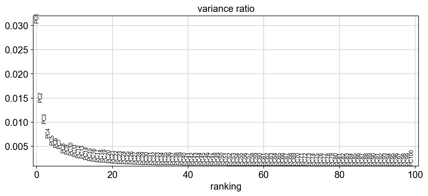
[11]:
sc.set_figure_params(figsize="10, 4")
sc.pl.pca_variance_ratio(adM1Norm, 100)
[12]:
npcs = 15
nknns = 15
sc.pp.neighbors(adM1Norm, n_neighbors=nknns, n_pcs=npcs)
sc.tl.leiden(adM1Norm,.25)
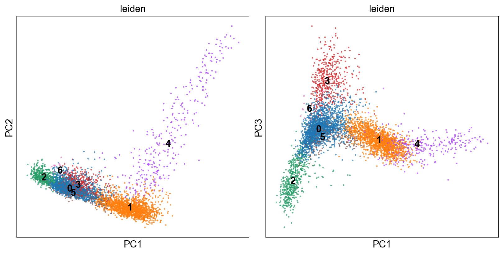
[13]:
fig, axs = plt.subplots(1,2, figsize=(10,5), constrained_layout=True)
sc.pl.pca(adM1Norm, color=["leiden"], alpha=.7, s=20, components="1,2",legend_loc='on data', ax=axs[0], show=False)
sc.pl.pca(adM1Norm, color=["leiden"], alpha=.7, s=20, components="1,3",legend_loc='on data', ax=axs[1], show=False)
... storing 'sampleName' as categorical
[13]:
<AxesSubplot:title={'center':'leiden'}, xlabel='PC1', ylabel='PC3'>
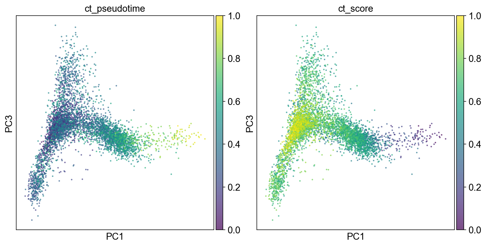
[14]:
fig, axs = plt.subplots(1,2, figsize=(10,5), constrained_layout=True)
sc.pl.pca(adM1Norm, color=["ct_pseudotime"], alpha=.7, s=20, components="1,3",legend_loc='on data', ax=axs[0], show=False)
sc.pl.pca(adM1Norm, color=["ct_score"], alpha=.7, s=20, components="1,3",legend_loc='on data', ax=axs[1], show=False)
[14]:
<AxesSubplot:title={'center':'ct_score'}, xlabel='PC1', ylabel='PC3'>
[15]:
adM1X = adM1Norm[adM1Norm.obs['leiden'] != "6"].copy()
adM1X = adM1X[adM1X.obs['leiden'] != "5"].copy()
adM1X
[15]:
AnnData object with n_obs × n_vars = 4894 × 15687
    obs: 'sampleName', 'n_genes_by_counts', 'total_counts', 'total_counts_ribo', 'pct_counts_ribo', 'total_counts_mt', 'pct_counts_mt', 'n_counts', 'ct_num_exp_genes', 'ct_score', 'ct_pseudotime', 'leiden'
    var: 'gene_ids', 'mt', 'ribo', 'n_cells_by_counts', 'mean_counts', 'pct_dropout_by_counts', 'total_counts', 'n_cells', 'highly_variable', 'means', 'dispersions', 'dispersions_norm', 'ct_gene_corr', 'ct_correlates', 'mean', 'std'
    uns: 'log1p', 'hvg', 'pca', 'neighbors', 'ct_params', 'leiden', 'leiden_colors'
    obsm: 'X_pca'
    varm: 'PCs'
    layers: 'spliced', 'unspliced', 'Ms', 'Mu'
    obsp: 'distances', 'connectivities'
[16]:
sc.tl.rank_genes_groups(adM1X, 'leiden')
sc.pl.rank_genes_groups_dotplot(adM1X, n_genes=8, groupby='leiden', use_raw=False, dendrogram=False)
WARNING: Default of the method has been changed to 't-test' from 't-test_overestim_var'
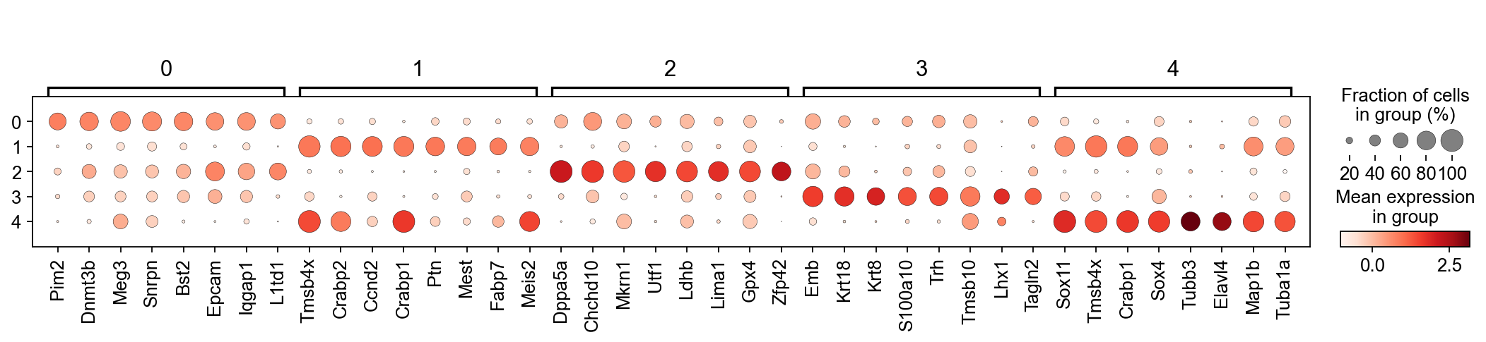
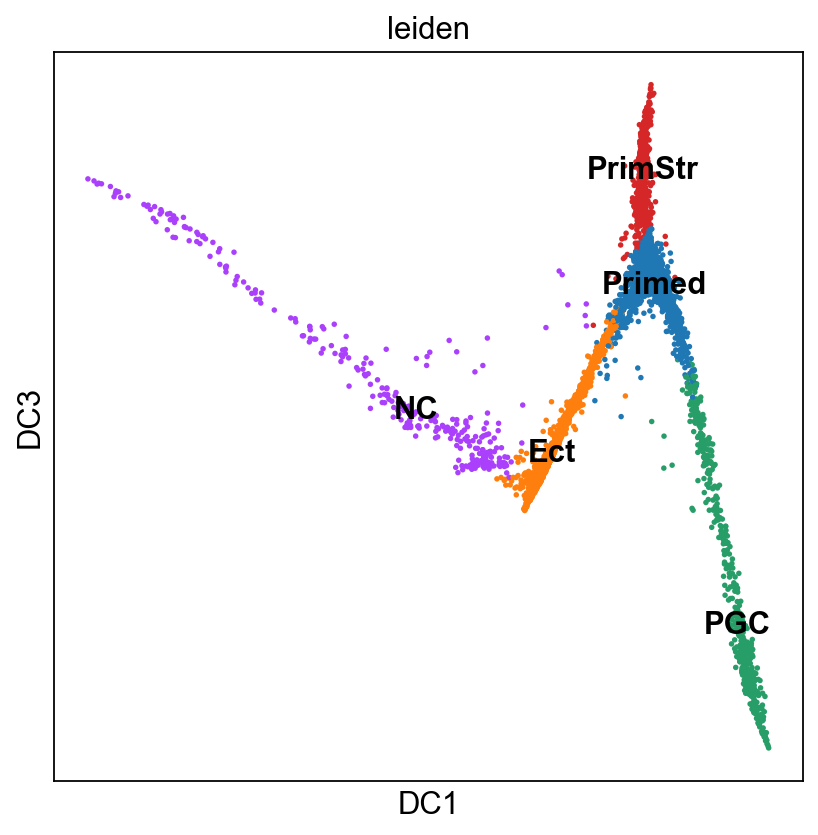
Based on this and what we found out on Tues, I think the following cluster annotation makes sense:
Primed
Ect
PGC
PrimStr
NC
Let’s rename the clusters
[17]:
new_sc_names = ["Primed","Ect", "PGC", "PrimStr", "NC"]
adM1X.rename_categories('leiden', new_sc_names)
[18]:
sc.tl.diffmap(adM1X)
[19]:
sc.set_figure_params(figsize="6,6")
sc.pl.diffmap(adM1X, color="leiden", components=["1,3"], legend_loc="on data")
[20]:
adM1X.uns['iroot'] = np.flatnonzero(adM1X.obs['leiden']  == 'Primed')[0]

sc.tl.dpt(adM1X)
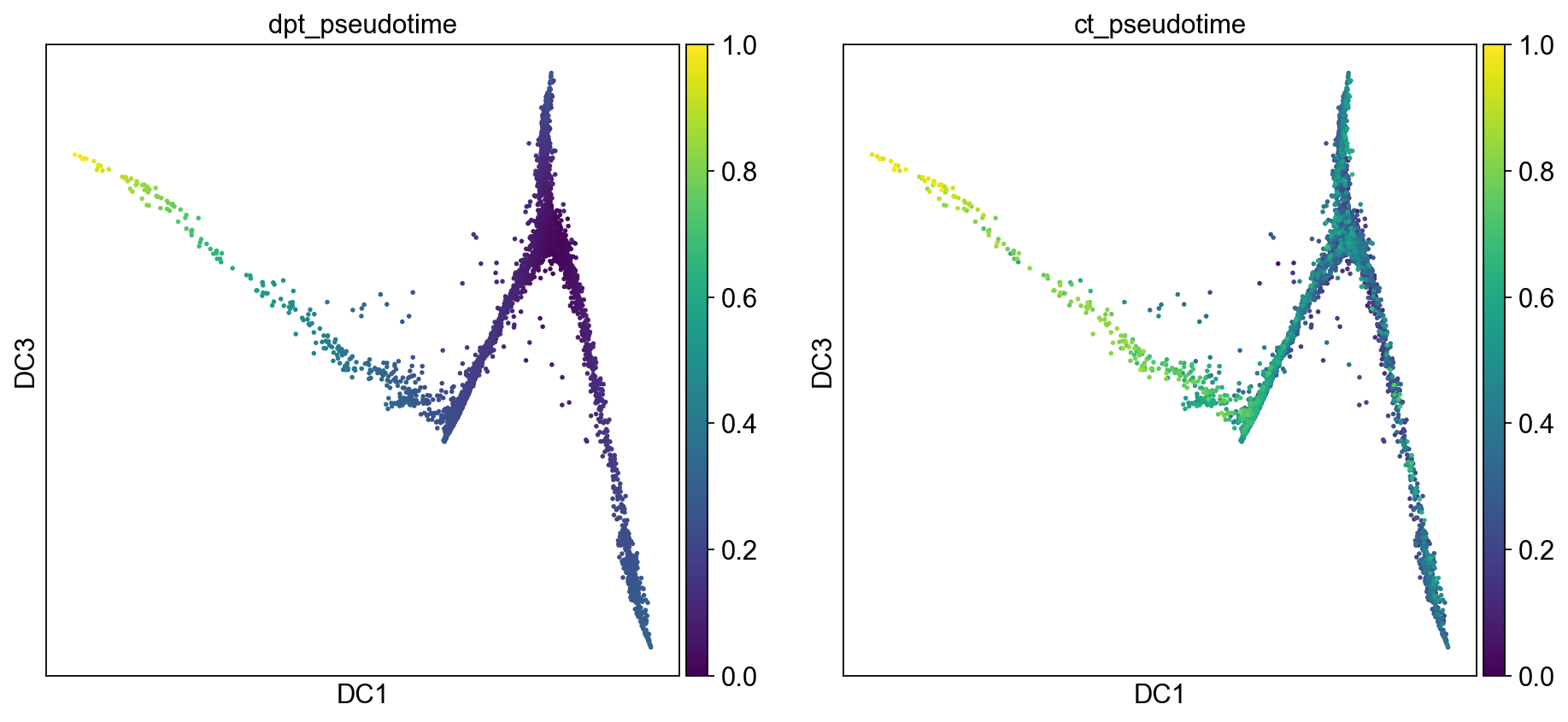
[21]:
sc.pl.diffmap(adM1X, color=["dpt_pseudotime","ct_pseudotime"], components=("1,3"), legend_loc='on data')
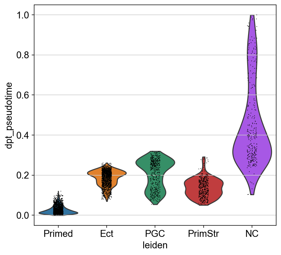
[22]:
sc.pl.violin(adM1X, "dpt_pseudotime", groupby="leiden")
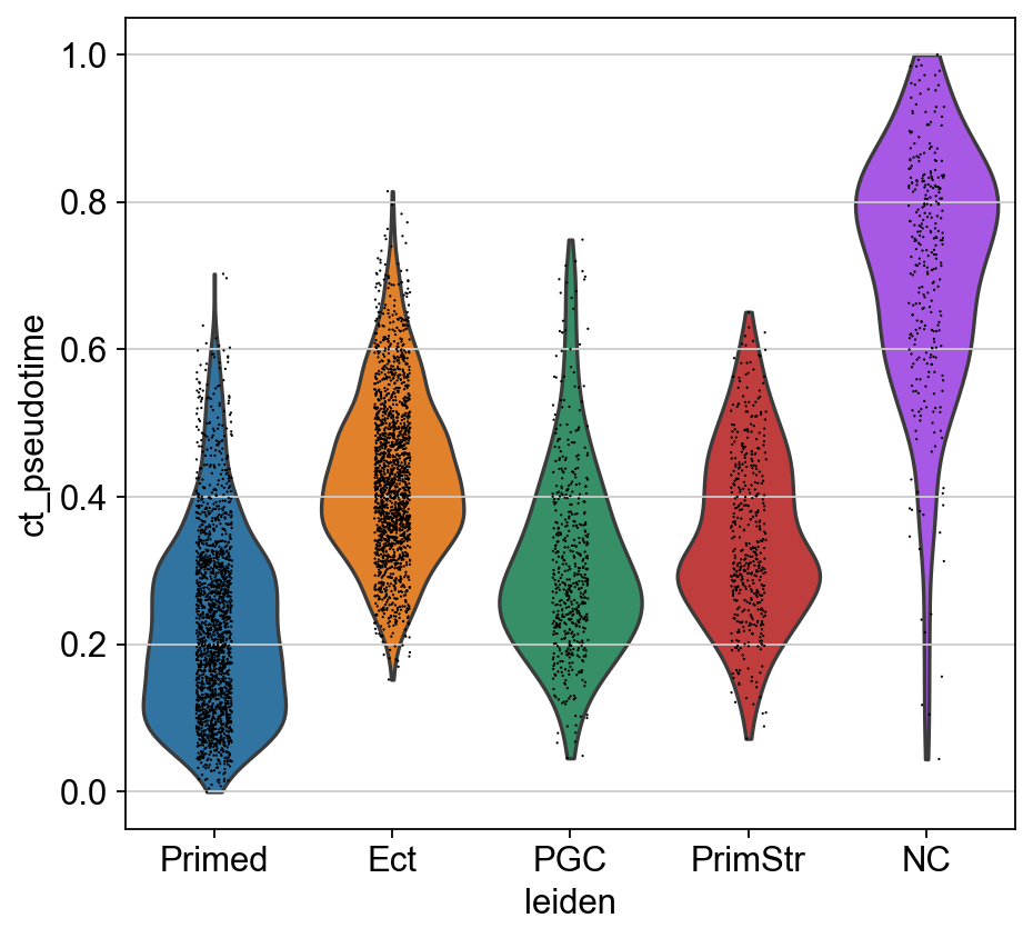
[23]:
sc.pl.violin(adM1X, "ct_pseudotime", groupby="leiden")
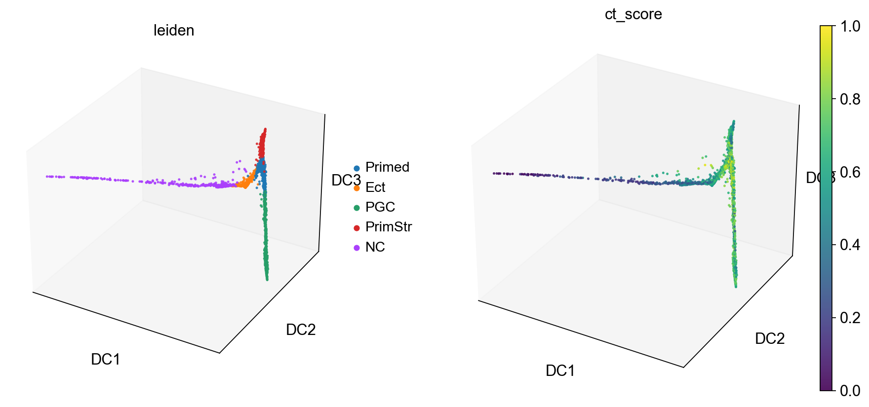
[24]:
sc.pl.diffmap(adM1X, color=["leiden", "ct_score"], alpha=.9, s=35, projection='3d')
[ ]: