RNA velocity analysis
This walk-thru is based heavily on https://scvelo.readthedocs.io/VelocityBasics/
[1]:
import pandas as pd
import matplotlib.pyplot as plt
import seaborn as sns
import scanpy as sc
import scipy as sp
import numpy as np
import warnings
warnings.filterwarnings('ignore')

# NB these new packages
import scvelo as scv
import cellrank as cr
[2]:
scv.settings.presenter_view = True
scv.set_figure_params('scvelo')
Describe the first data set…
[3]:
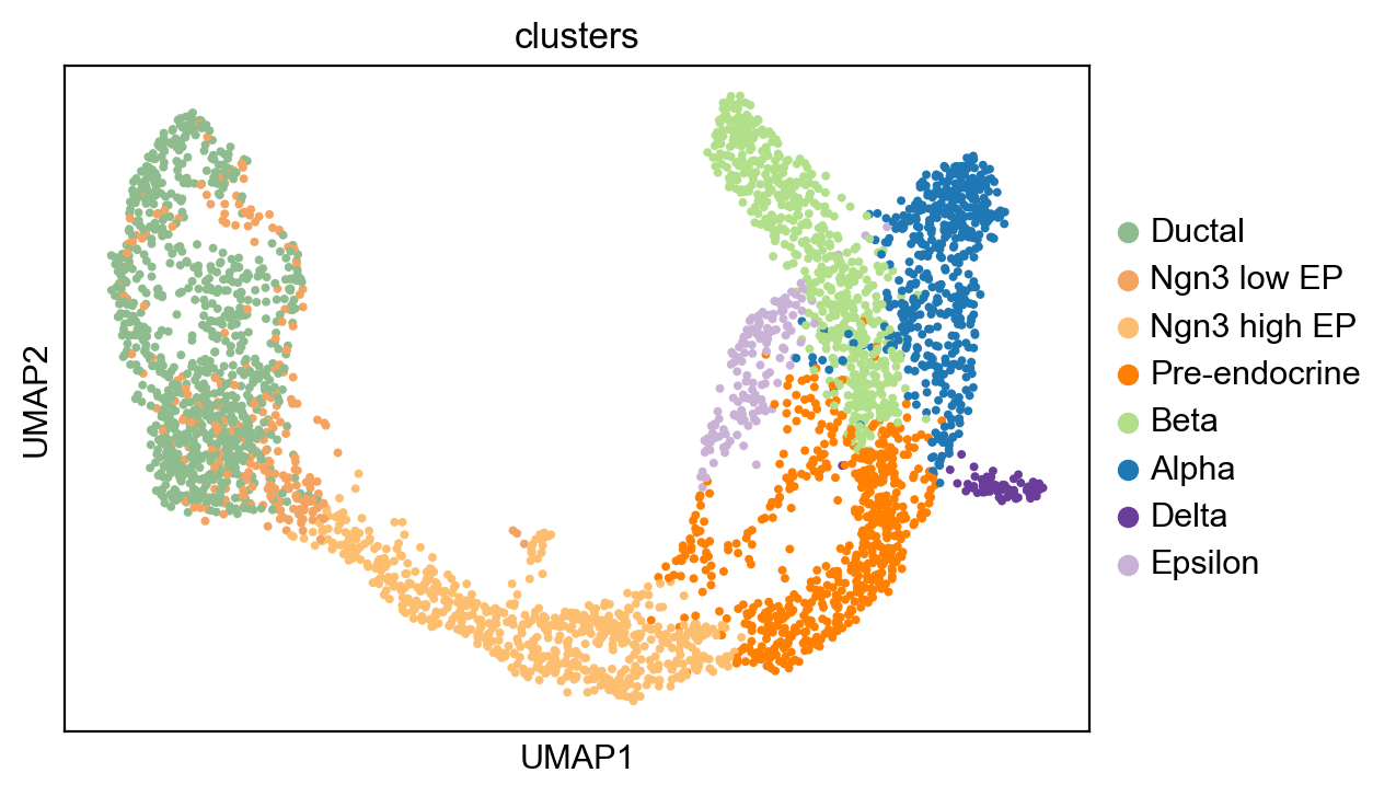
adata = scv.datasets.pancreas()
adata
[3]:
AnnData object with n_obs × n_vars = 3696 × 27998
    obs: 'clusters_coarse', 'clusters', 'S_score', 'G2M_score'
    var: 'highly_variable_genes'
    uns: 'clusters_coarse_colors', 'clusters_colors', 'day_colors', 'neighbors', 'pca'
    obsm: 'X_pca', 'X_umap'
    layers: 'spliced', 'unspliced'
    obsp: 'distances', 'connectivities'
[4]:
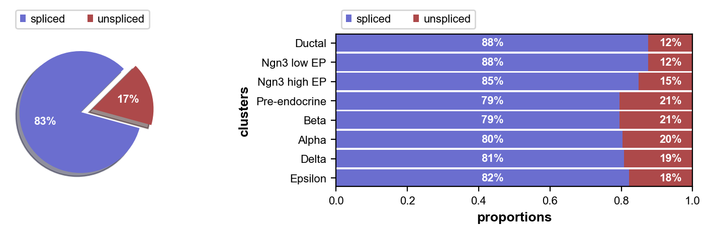
scv.pl.proportions(adata)
[5]:
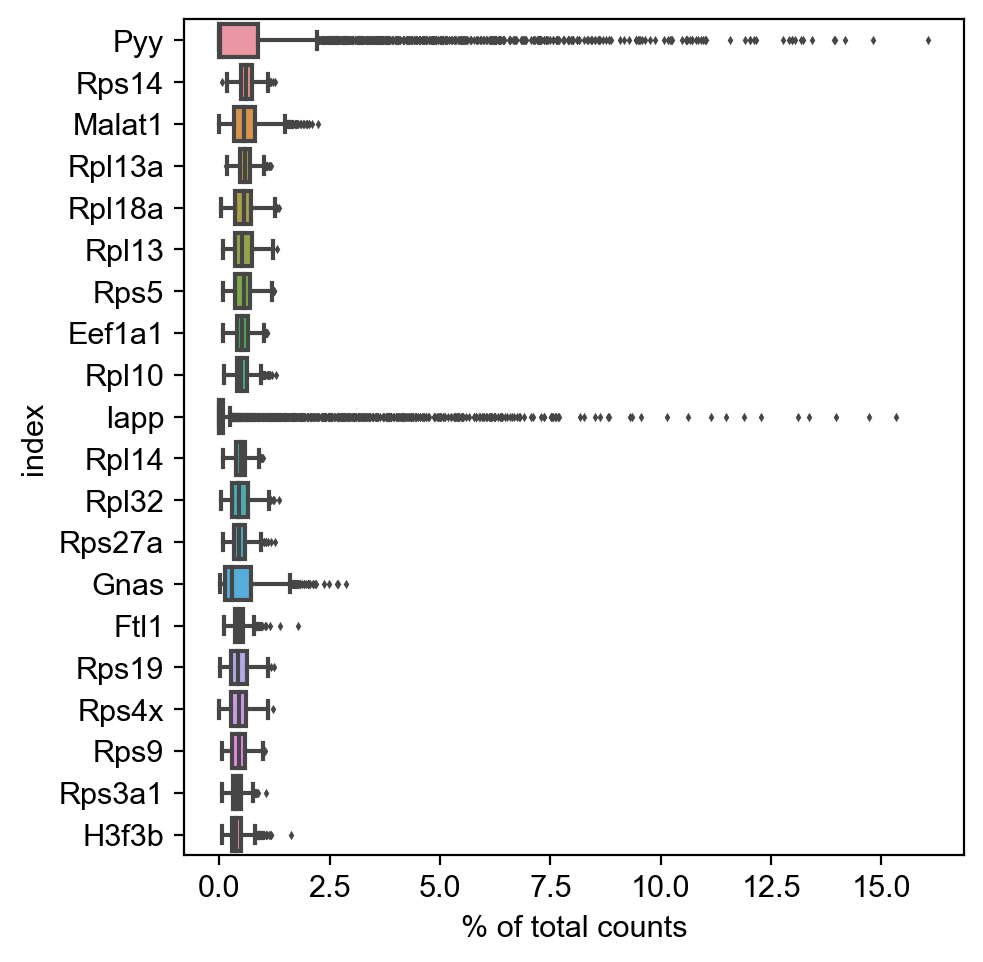
sc.pl.highest_expr_genes(adata, n_top=20, )
[6]:
adata.obs
[6]:
| clusters_coarse | clusters | S_score | G2M_score | |
|---|---|---|---|---|
| index | ||||
| AAACCTGAGAGGGATA | Pre-endocrine | Pre-endocrine | -0.224902 | -0.252071 |
| AAACCTGAGCCTTGAT | Ductal | Ductal | -0.014707 | -0.232610 |
| AAACCTGAGGCAATTA | Endocrine | Alpha | -0.171255 | -0.286834 |
| AAACCTGCATCATCCC | Ductal | Ductal | 0.599244 | 0.191243 |
| AAACCTGGTAAGTGGC | Ngn3 high EP | Ngn3 high EP | -0.179981 | -0.126030 |
| ... | ... | ... | ... | ... |
| TTTGTCAAGTGACATA | Pre-endocrine | Pre-endocrine | -0.235896 | -0.266101 |
| TTTGTCAAGTGTGGCA | Ngn3 high EP | Ngn3 high EP | 0.279374 | -0.204047 |
| TTTGTCAGTTGTTTGG | Ductal | Ductal | -0.045692 | -0.208907 |
| TTTGTCATCGAATGCT | Endocrine | Alpha | -0.240576 | -0.206865 |
| TTTGTCATCTGTTTGT | Endocrine | Epsilon | -0.136407 | -0.184763 |
3696 rows × 4 columns
[7]:
adata.var
[7]:
| highly_variable_genes | |
|---|---|
| index | |
| Xkr4 | False |
| Gm37381 | NaN |
| Rp1 | NaN |
| Rp1-1 | NaN |
| Sox17 | NaN |
| ... | ... |
| Gm28672 | NaN |
| Gm28670 | NaN |
| Gm29504 | NaN |
| Gm20837 | NaN |
| Erdr1 | True |
27998 rows × 1 columns
[8]:
adata.var['mt']= adata.var_names.str.startswith(("mt-"))
print(sum(adata.var['mt']))
13
[9]:
adata.var['ribo'] = adata.var_names.str.startswith(("Rps","Rpl"))
print(sum(adata.var['ribo']))
113
[10]:
sc.pp.calculate_qc_metrics(adata, qc_vars=['ribo', 'mt'], percent_top=None, log1p=False, inplace=True)
[11]:
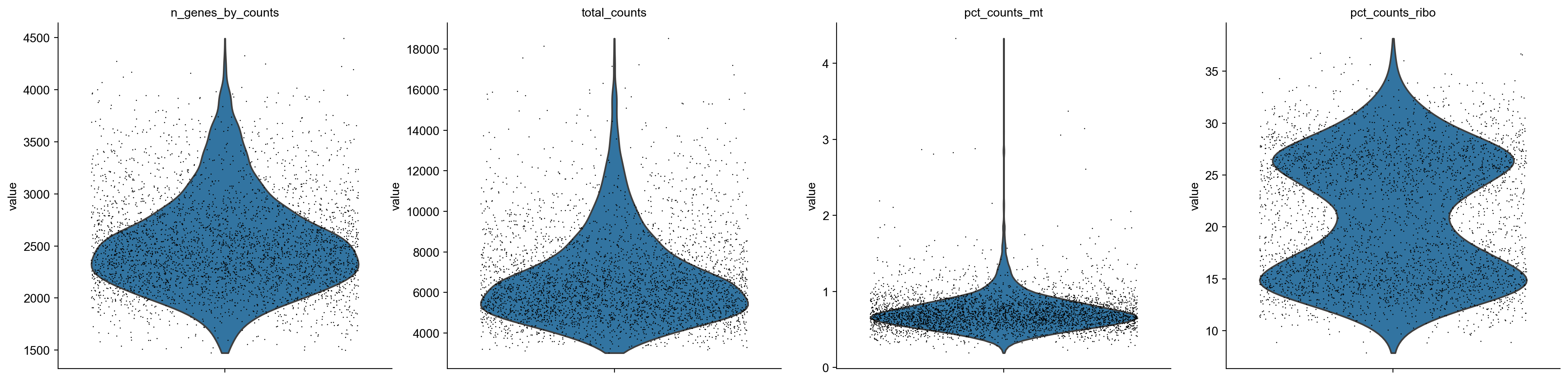
axs = sc.pl.violin(adata, ['n_genes_by_counts', 'total_counts', 'pct_counts_mt', 'pct_counts_ribo'],jitter=0.4, multi_panel=True)
[12]:
print("Number of genes: ",adata.n_vars)
gThresh = 5

sc.pp.filter_genes(adata, min_cells=gThresh)
print("Number of genes: ",adata.n_vars)
Number of genes:  27998
Number of genes:  14915
[13]:
mito_genes = adata.var_names.str.startswith('mt-')
ribo_genes = adata.var_names.str.startswith(("Rpl","Rps"))
malat_gene = adata.var_names.str.startswith("Malat1")

remove = np.add(mito_genes, ribo_genes)
remove = np.add(remove, malat_gene)

keep = np.invert(remove)
adata = adata[:,keep].copy()
print("Number of genes: ",adata.n_vars)
Number of genes: 14800
Spliced/unspliced normalization
[14]:
scv.pp.filter_genes(adata, min_shared_counts=20)
scv.pp.normalize_per_cell(adata)
scv.pp.filter_genes_dispersion(adata, n_top_genes=2000)
scv.pp.log1p(adata)
Filtered out 7692 genes that are detected 20 counts (shared).
Normalized count data: X, spliced, unspliced.
Extracted 2000 highly variable genes.
[15]:
adata
[15]:
AnnData object with n_obs × n_vars = 3696 × 2000
    obs: 'clusters_coarse', 'clusters', 'S_score', 'G2M_score', 'n_genes_by_counts', 'total_counts', 'total_counts_ribo', 'pct_counts_ribo', 'total_counts_mt', 'pct_counts_mt', 'initial_size_spliced', 'initial_size_unspliced', 'initial_size', 'n_counts'
    var: 'highly_variable_genes', 'mt', 'ribo', 'n_cells_by_counts', 'mean_counts', 'pct_dropout_by_counts', 'total_counts', 'n_cells', 'gene_count_corr', 'means', 'dispersions', 'dispersions_norm', 'highly_variable'
    uns: 'clusters_coarse_colors', 'clusters_colors', 'day_colors', 'neighbors', 'pca'
    obsm: 'X_pca', 'X_umap'
    layers: 'spliced', 'unspliced'
    obsp: 'distances', 'connectivities'
Smoothing
[17]:
# scv.pp.filter_and_normalize(adata, min_shared_counts=20, n_top_genes=2000) <- this will do the same thing as lines above
scv.pp.moments(adata, n_pcs=30, n_neighbors=30)
adata
computing neighbors
OMP: Info #271: omp_set_nested routine deprecated, please use omp_set_max_active_levels instead.
    finished (0:00:06) --> added
    'distances' and 'connectivities', weighted adjacency matrices (adata.obsp)
computing moments based on connectivities
    finished (0:00:00) --> added
    'Ms' and 'Mu', moments of un/spliced abundances (adata.layers)
[17]:
AnnData object with n_obs × n_vars = 3696 × 2000
    obs: 'clusters_coarse', 'clusters', 'S_score', 'G2M_score', 'n_genes_by_counts', 'total_counts', 'total_counts_ribo', 'pct_counts_ribo', 'total_counts_mt', 'pct_counts_mt', 'initial_size_spliced', 'initial_size_unspliced', 'initial_size', 'n_counts'
    var: 'highly_variable_genes', 'mt', 'ribo', 'n_cells_by_counts', 'mean_counts', 'pct_dropout_by_counts', 'total_counts', 'n_cells', 'gene_count_corr', 'means', 'dispersions', 'dispersions_norm', 'highly_variable'
    uns: 'clusters_coarse_colors', 'clusters_colors', 'day_colors', 'neighbors', 'pca'
    obsm: 'X_pca', 'X_umap'
    layers: 'spliced', 'unspliced', 'Ms', 'Mu'
    obsp: 'distances', 'connectivities'
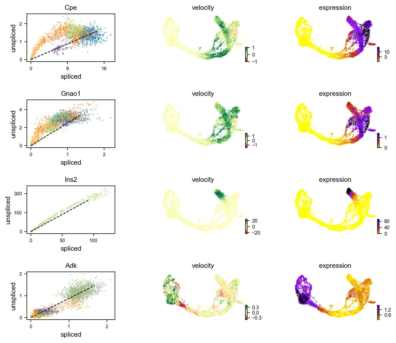
Finally compute velocity
walk thru phase plot below
[18]:
scv.tl.velocity(adata)
computing velocities
    finished (0:00:01) --> added
    'velocity', velocity vectors for each individual cell (adata.layers)
[19]:
adata
[19]:
AnnData object with n_obs × n_vars = 3696 × 2000
    obs: 'clusters_coarse', 'clusters', 'S_score', 'G2M_score', 'n_genes_by_counts', 'total_counts', 'total_counts_ribo', 'pct_counts_ribo', 'total_counts_mt', 'pct_counts_mt', 'initial_size_spliced', 'initial_size_unspliced', 'initial_size', 'n_counts'
    var: 'highly_variable_genes', 'mt', 'ribo', 'n_cells_by_counts', 'mean_counts', 'pct_dropout_by_counts', 'total_counts', 'n_cells', 'gene_count_corr', 'means', 'dispersions', 'dispersions_norm', 'highly_variable', 'velocity_gamma', 'velocity_qreg_ratio', 'velocity_r2', 'velocity_genes'
    uns: 'clusters_coarse_colors', 'clusters_colors', 'day_colors', 'neighbors', 'pca', 'velocity_params'
    obsm: 'X_pca', 'X_umap'
    layers: 'spliced', 'unspliced', 'Ms', 'Mu', 'velocity', 'variance_velocity'
    obsp: 'distances', 'connectivities'
Transition matrix
for embedding
for velocity pt
[20]:
scv.tl.velocity_graph(adata)
computing velocity graph (using 1/8 cores)
/Users/patrickcahan/opt/anaconda3/lib/python3.9/site-packages/scvelo/core/_parallelize.py:138: VisibleDeprecationWarning: Creating an ndarray from ragged nested sequences (which is a list-or-tuple of lists-or-tuples-or ndarrays with different lengths or shapes) is deprecated. If you meant to do this, you must specify 'dtype=object' when creating the ndarray.
  res = np.array(res) if as_array else res
    finished (0:00:21) --> added
    'velocity_graph', sparse matrix with cosine correlations (adata.uns)
Placing velocities onto embedding
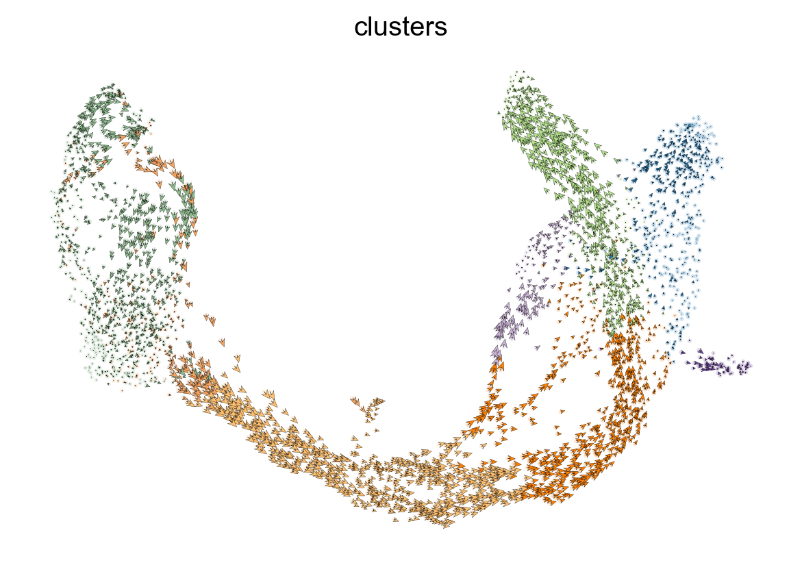
[21]:
scv.pl.velocity_embedding(adata, arrow_length=3, arrow_size=2, dpi=120)
computing velocity embedding
    finished (0:00:00) --> added
    'velocity_umap', embedded velocity vectors (adata.obsm)
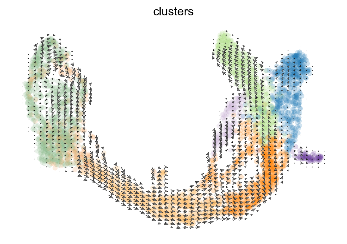
[22]:
scv.pl.velocity_embedding_grid(adata, arrow_length=3, arrow_size=2, dpi=120)
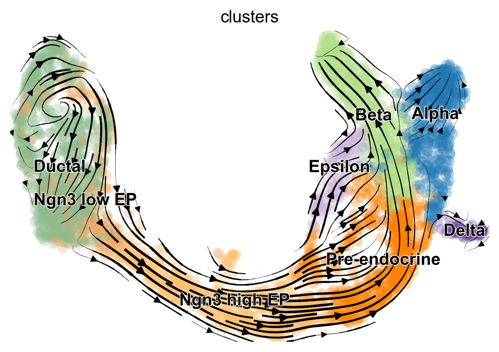
[23]:
scv.pl.velocity_embedding_stream(adata, basis='umap')
Still just an annData, so we can do the usual things
[24]:
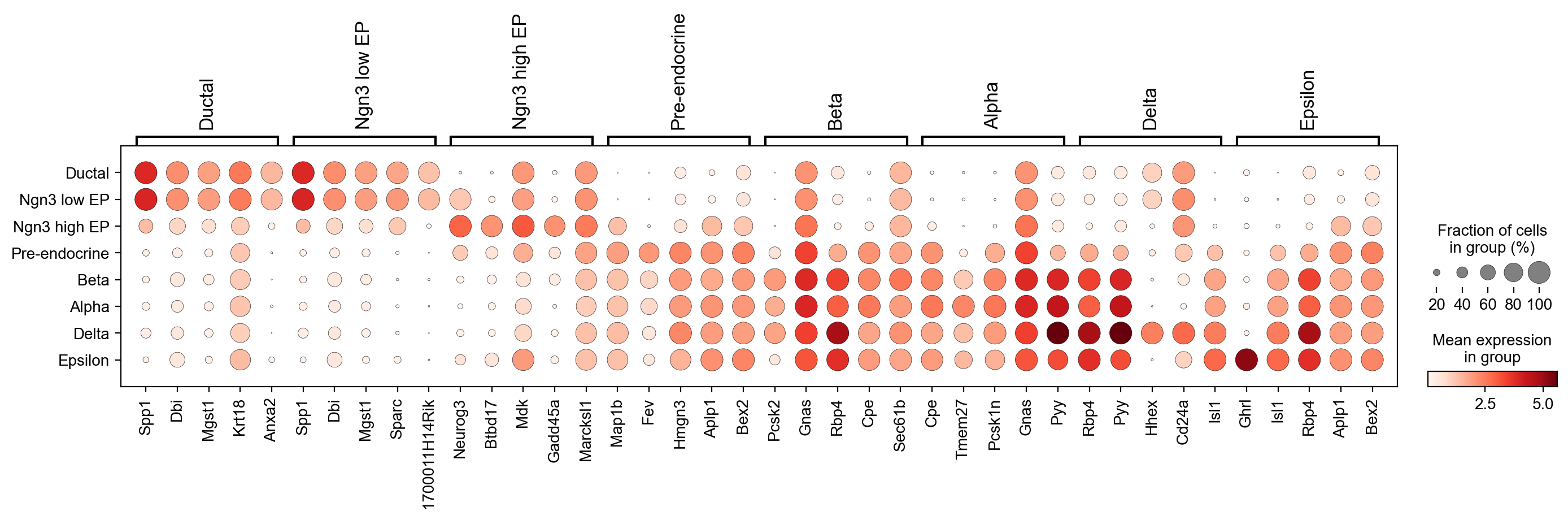
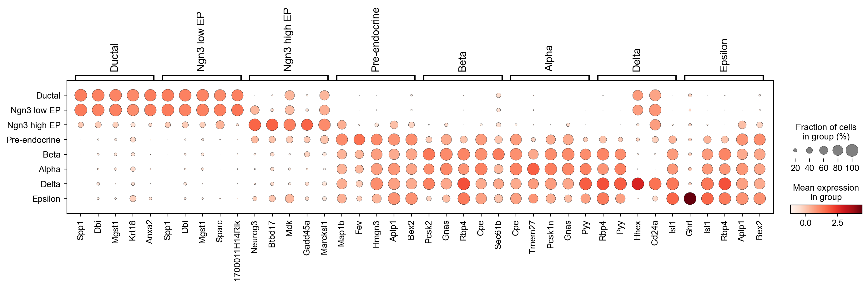
sc.tl.rank_genes_groups(adata,'clusters', use_raw=False)
sc.pl.rank_genes_groups_dotplot(adata, n_genes=5, groupby='clusters', use_raw=False, dendrogram=False)
WARNING: Default of the method has been changed to 't-test' from 't-test_overestim_var'
[25]:
sc.pp.scale(adata, max_value=10)
[26]:
sc.tl.rank_genes_groups(adata,'clusters', use_raw=False)
sc.pl.rank_genes_groups_dotplot(adata, n_genes=5, groupby='clusters', use_raw=False, dendrogram=False)
WARNING: Default of the method has been changed to 't-test' from 't-test_overestim_var'
Find genes whose velocities differ between clusters
[28]:
scv.tl.rank_velocity_genes(adata, groupby='clusters', min_corr=.3)

df = scv.DataFrame(adata.uns['rank_velocity_genes']['names'])
df.head()
ranking velocity genes
    finished (0:00:02) --> added
    'rank_velocity_genes', sorted scores by group ids (adata.uns)
    'spearmans_score', spearmans correlation scores (adata.var)
[28]:
| Ductal | Ngn3 low EP | Ngn3 high EP | Pre-endocrine | Beta | Alpha | Delta | Epsilon | |
|---|---|---|---|---|---|---|---|---|
| 0 | 2610035D17Rik | 2610035D17Rik | Pde1c | Pam | Pax6 | Zcchc16 | Zdbf2 | Heg1 |
| 1 | Notch2 | Hivep2 | Ptprs | Sdk1 | Unc5c | Nlgn1 | Akr1c19 | Tmcc3 |
| 2 | Gm20649 | Gm20649 | Ttyh2 | Abcc8 | Nnat | Nell1 | Spock3 | Ica1 |
| 3 | Sox5 | Gulp1 | Pclo | Baiap3 | Tmem108 | Chrm3 | Ptprt | Ncoa7 |
| 4 | Naaladl2 | Echdc2 | Grik2 | Gnas | Ptprt | Prune2 | Snap25 | Ank2 |
[29]:
scv.pl.velocity(adata, ["Sox5", "Hivep2", "Ptprs", "Pam", "Pax6", "Ins1"], ncols=1)
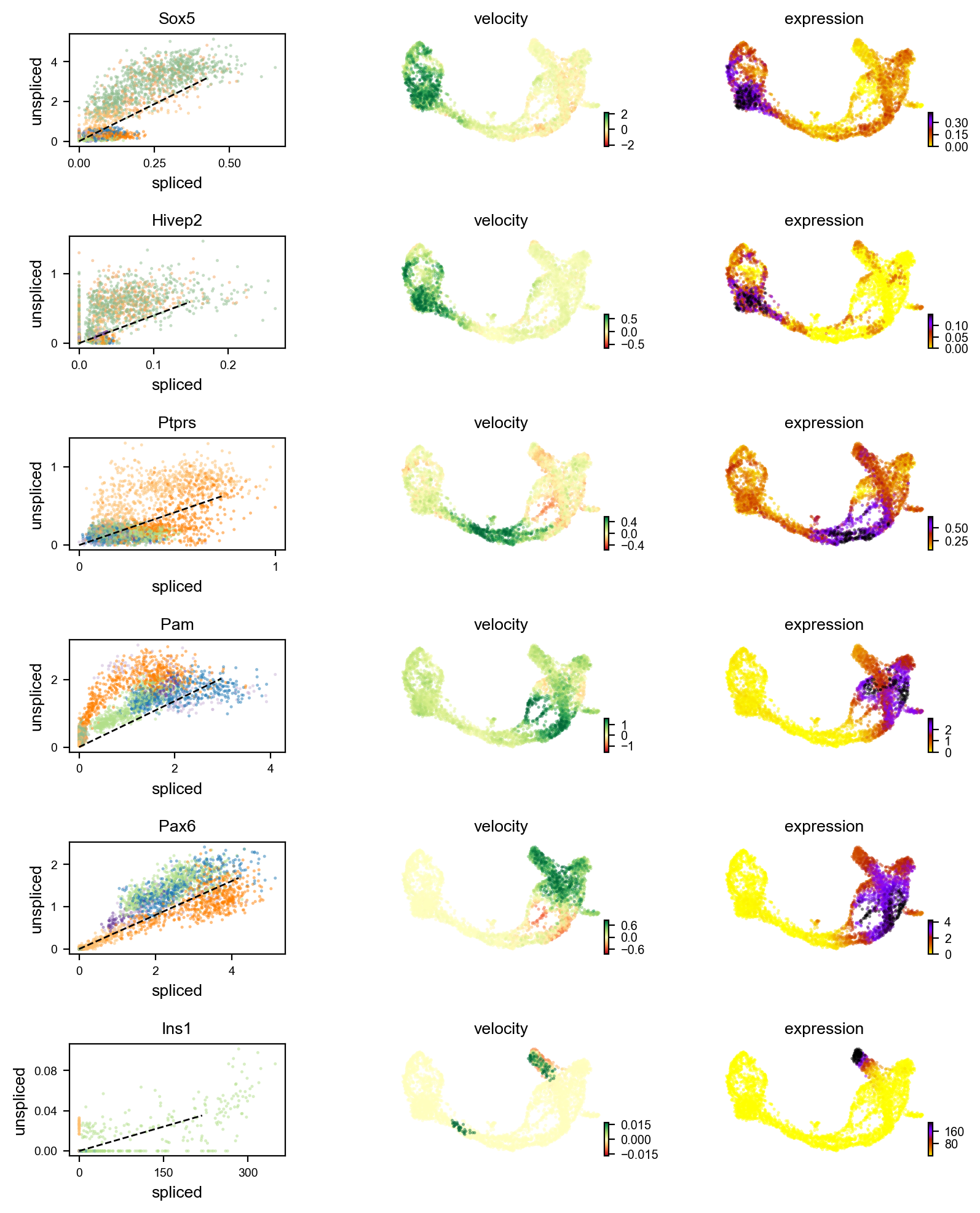
Does Ins1 have introns? Show students Entrez Gene, and how to view the gene structure.
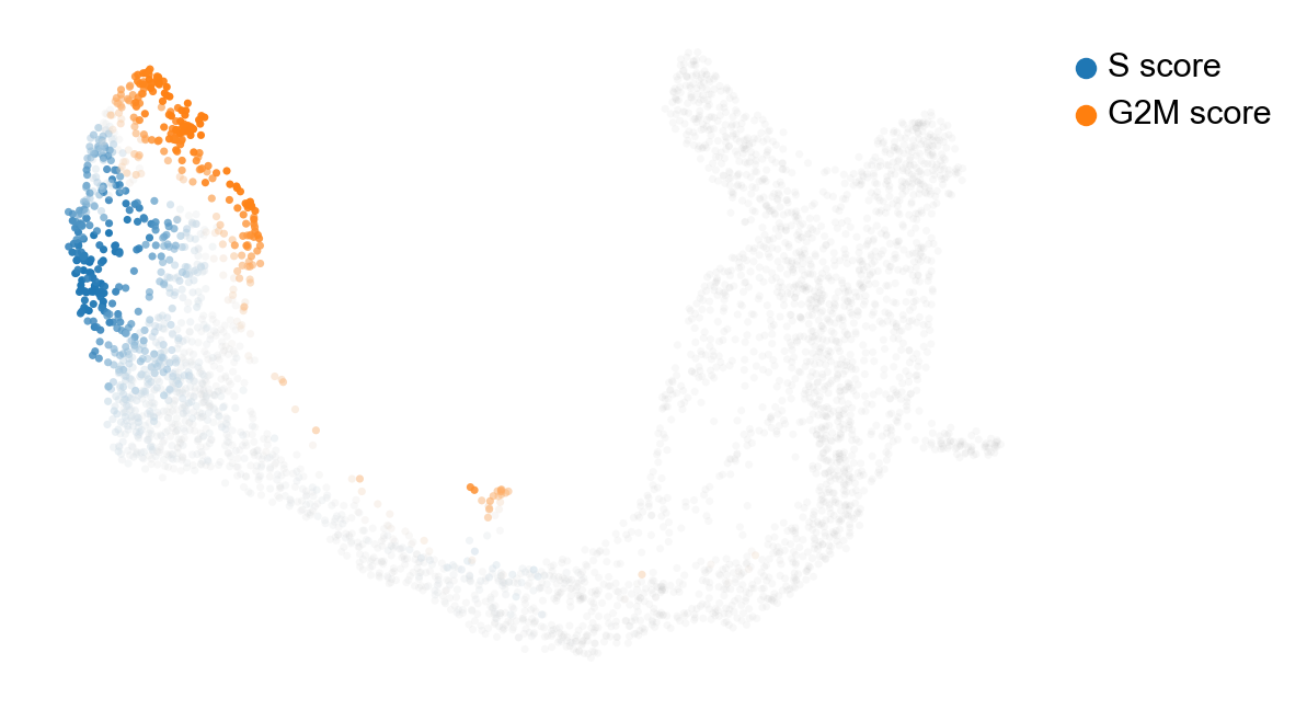
Cell cycle
What is the cycle in the ductal compartment???
[30]:
scv.tl.score_genes_cell_cycle(adata)
calculating cell cycle phase
-->     'S_score' and 'G2M_score', scores of cell cycle phases (adata.obs)
[31]:
scv.pl.scatter(adata, color_gradients=['S_score', 'G2M_score'], smooth=True, perc=[5, 95])
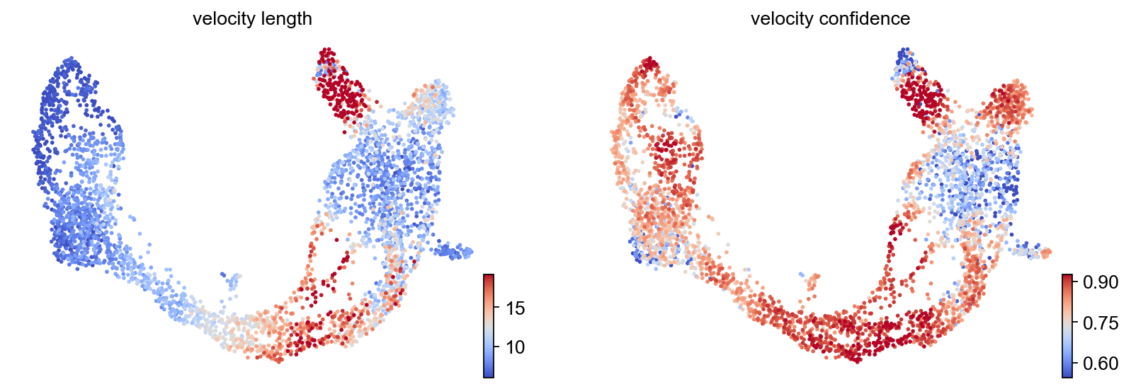
Magnitude and “confidence”
explain these metrics and what ‘confidence’ in this context really means
[32]:
scv.tl.velocity_confidence(adata)
keys = 'velocity_length', 'velocity_confidence'
scv.pl.scatter(adata, c=keys, cmap='coolwarm', perc=[5, 95])
--> added 'velocity_length' (adata.obs)
--> added 'velocity_confidence' (adata.obs)
--> added 'velocity_confidence_transition' (adata.obs)
Cluster analysis of state transitions
[33]:
df = adata.obs.groupby('clusters')[keys].mean().T
df.style.background_gradient(cmap='coolwarm', axis=1)
[33]:
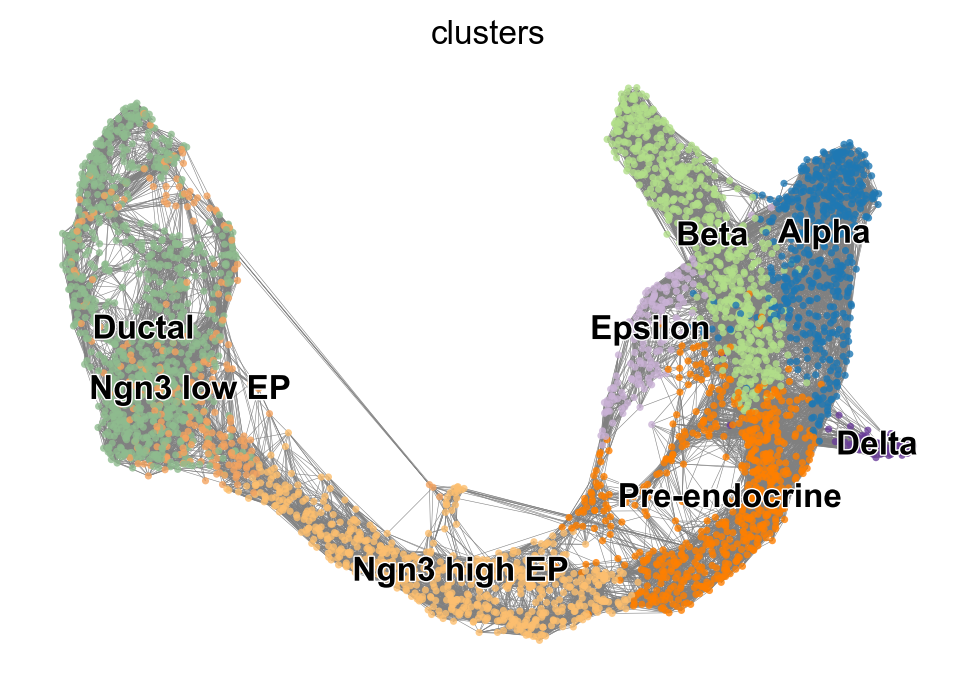
| clusters | Ductal | Ngn3 low EP | Ngn3 high EP | Pre-endocrine | Beta | Alpha | Delta | Epsilon |
|---|---|---|---|---|---|---|---|---|
| velocity_length | 7.249028 | 7.729008 | 13.006619 | 12.847837 | 14.069593 | 9.907110 | 7.749000 | 10.523310 |
| velocity_confidence | 0.793872 | 0.770499 | 0.875152 | 0.805025 | 0.709603 | 0.727740 | 0.698432 | 0.782908 |
How are cells predicted to be related to each other? Look at transition matrix
[34]:
scv.pl.velocity_graph(adata, threshold=.1)
What is the ultimate fate of a given cell?
[35]:
x, y = scv.utils.get_cell_transitions(adata, basis='umap', starting_cell=70)
ax = scv.pl.velocity_graph(adata, c='lightgrey', edge_width=.05, show=False)
ax = scv.pl.scatter(adata, x=x, y=y, s=120, c='ascending', cmap='gnuplot', ax=ax)
[ ]:
x, y = scv.utils.get_cell_transitions(adata, basis='umap', starting_cell=1001)
ax = scv.pl.velocity_graph(adata, c='lightgrey', edge_width=.05, show=False)
ax = scv.pl.scatter(adata, x=x, y=y, s=120, c='ascending', cmap='gnuplot', ax=ax)
[36]:
x, y = scv.utils.get_cell_transitions(adata, basis='umap', starting_cell=11)
ax = scv.pl.velocity_graph(adata, c='lightgrey', edge_width=.05, show=False)
ax = scv.pl.scatter(adata, x=x, y=y, s=120, c='ascending', cmap='gnuplot', ax=ax)
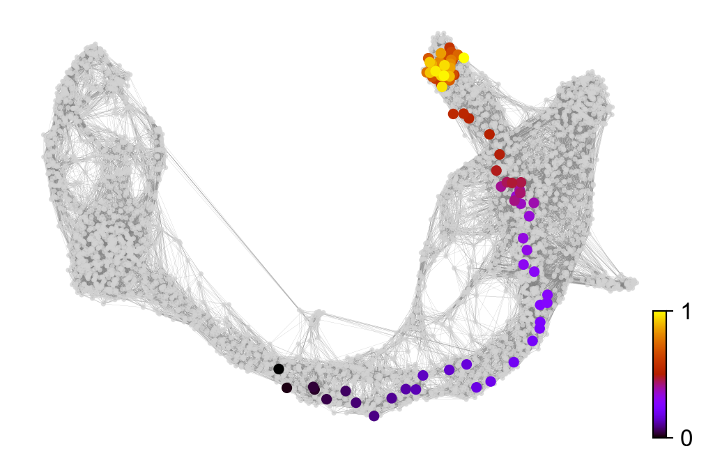
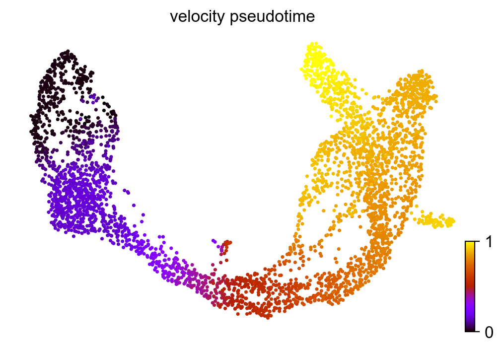
Velocity pseudotime
[37]:
scv.tl.velocity_pseudotime(adata)
scv.pl.scatter(adata, color='velocity_pseudotime', cmap='gnuplot')
computing terminal states
    identified 2 regions of root cells and 1 region of end points .
    finished (0:00:00) --> added
    'root_cells', root cells of Markov diffusion process (adata.obs)
    'end_points', end points of Markov diffusion process (adata.obs)
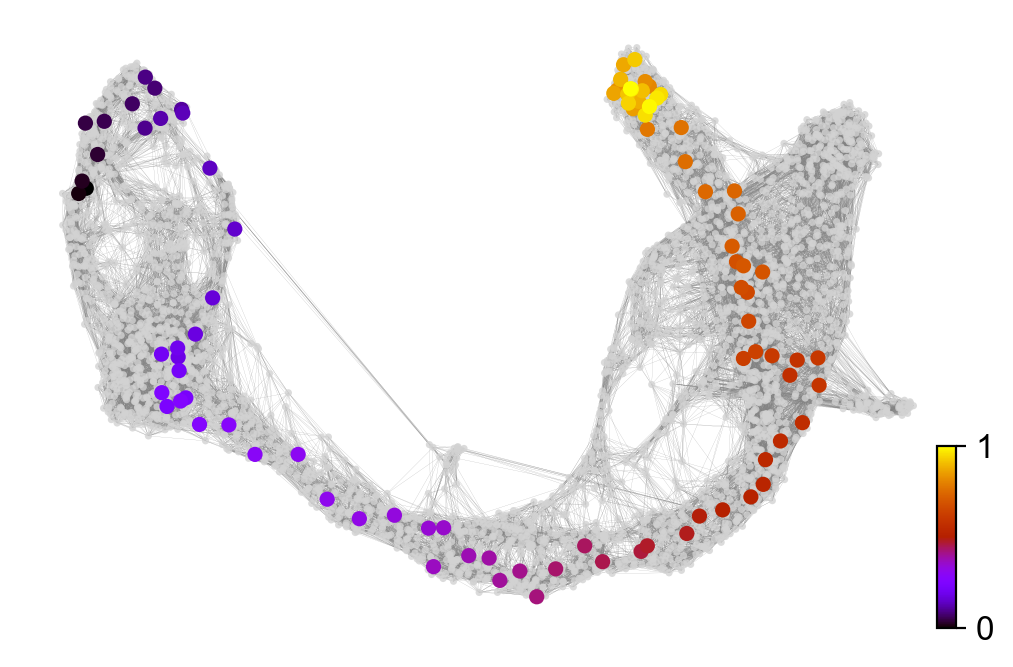
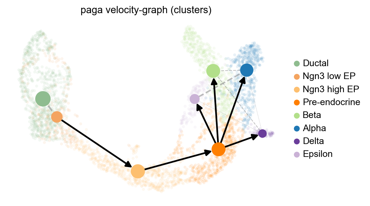
Again, aggregate these transitions to a cluster level with PAGA
[38]:
adata.uns['neighbors']['distances'] = adata.obsp['distances']
adata.uns['neighbors']['connectivities'] = adata.obsp['connectivities']

scv.tl.paga(adata, groups='clusters')
df = scv.get_df(adata, 'paga/transitions_confidence', precision=2).T
df.style.background_gradient(cmap='Blues').format('{:.2g}')
running PAGA using priors: ['velocity_pseudotime']
    finished (0:00:01) --> added
    'paga/connectivities', connectivities adjacency (adata.uns)
    'paga/connectivities_tree', connectivities subtree (adata.uns)
    'paga/transitions_confidence', velocity transitions (adata.uns)
[38]:
| Ductal | Ngn3 low EP | Ngn3 high EP | Pre-endocrine | Beta | Alpha | Delta | Epsilon | |
|---|---|---|---|---|---|---|---|---|
| Ductal | 0 | 0 | 0.024 | 0 | 0 | 0 | 0 | 0 |
| Ngn3 low EP | 0 | 0 | 0.24 | 0 | 0 | 0 | 0 | 0 |
| Ngn3 high EP | 0 | 0 | 0 | 0.23 | 0 | 0 | 0 | 0 |
| Pre-endocrine | 0 | 0 | 0 | 0 | 0.5 | 0.098 | 0.21 | 0.12 |
| Beta | 0 | 0 | 0 | 0 | 0 | 0 | 0 | 0 |
| Alpha | 0 | 0 | 0 | 0 | 0 | 0 | 0 | 0 |
| Delta | 0 | 0 | 0 | 0 | 0 | 0 | 0 | 0 |
| Epsilon | 0 | 0 | 0 | 0 | 0 | 0 | 0 | 0 |
[39]:
scv.pl.paga(adata, basis='umap', size=50, alpha=.1,
            min_edge_width=2, node_size_scale=1.5)
[ ]: